Peptide AEDL alters chromatin conformation via histone binding

Larisa I. Fedoreyeva; Boris F. Vanyushin; Ekaterina N. Baranova; Larisa I. Fedoreyeva; Boris F. Vanyushin; Ekaterina N. Baranova

doi:10.3934/biophy.2020001

AIMS Biophysics

2020, Volume 7, Issue 1: 1-16. doi: 10.3934/biophy.2020001

Previous Article Next Article

Research article Special Issues

Peptide AEDL alters chromatin conformation via histone binding

1.
A.N.Belozersky Institute of Physico-Chemical Biology, Lomonosov Moscow State University, 119991 Moscow, Leninskie Gory1, building 40
2.
All-Russian Research Institute of Agricultural Biotechnology RAS, 127550 Moscow, Timiryazevskaya 42

Received: 01 November 2019 Accepted: 31 January 2020 Published: 06 February 2020

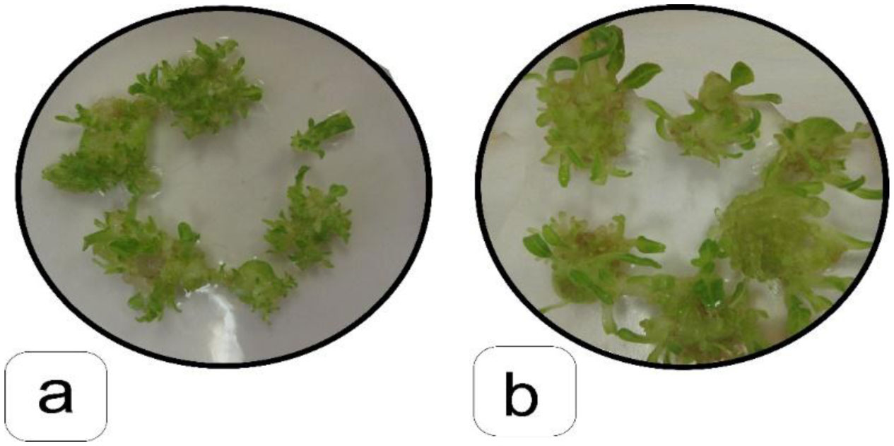
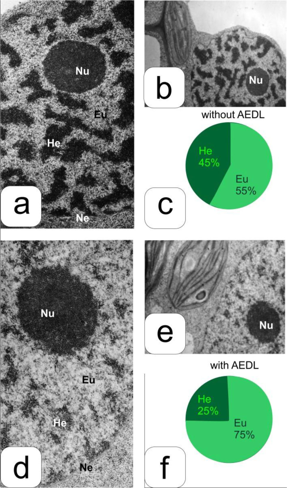
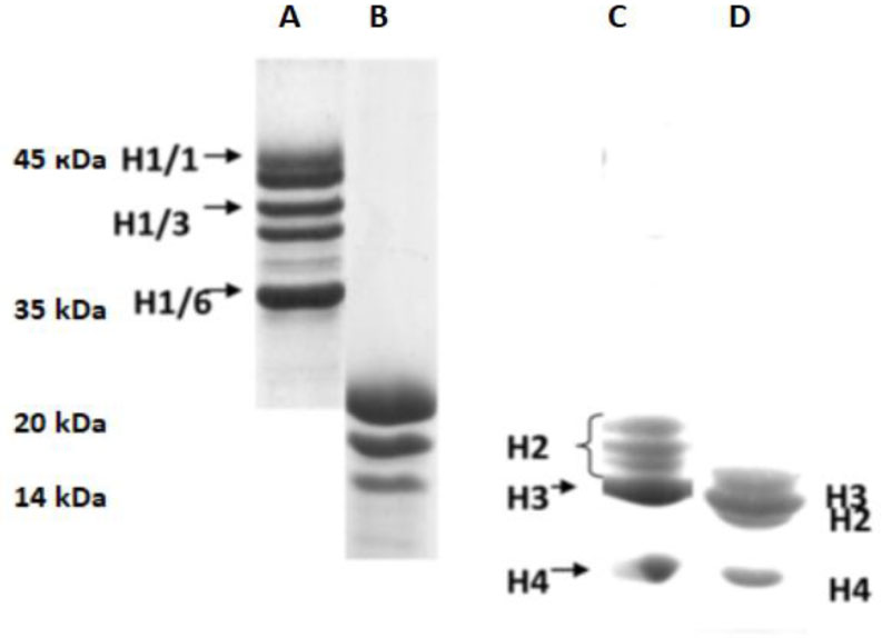
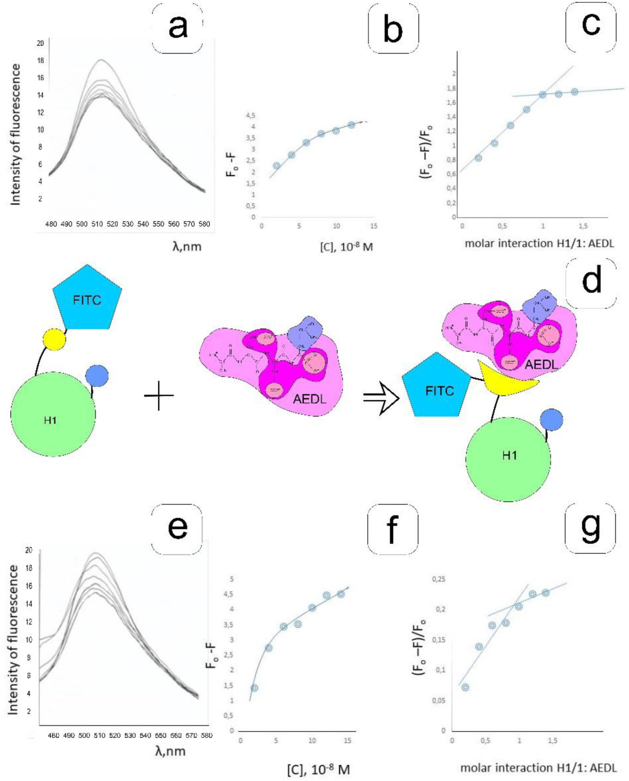
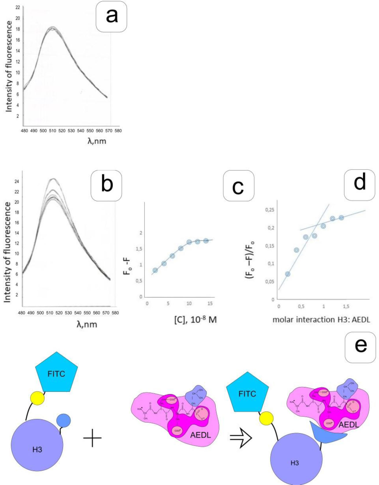
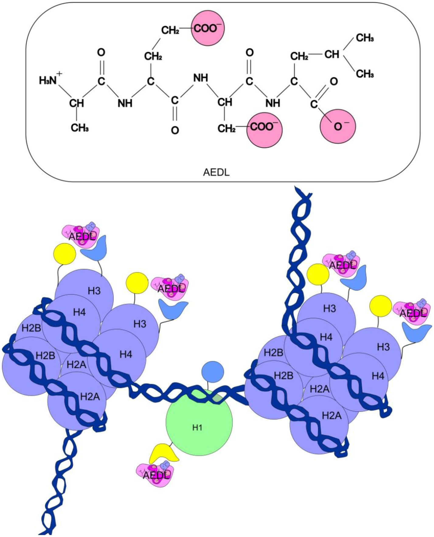
Eukaryotic DNA is tightly packed into chromatin, a DNA–protein structure that exists as transcriptionally permissive euchromatin or repressive heterochromatin. Post-translational modification of histones plays a key role in regulating chromatin dynamics. Short peptides derived from various sources are known to function as epigenetic modulators; however, their mechanisms of action are poorly understood. We addressed this issued by investigating the effect of peptide AEDL on chromatin structure in tobacco (Nicotiana tabacum L.), a commercially important plant species. The chromatin of tobacco interphase cells is characterized by the presence of zones of transcriptionally active domains and particular domains of condensed chromatin of cells that partially coincide with heterochromatin zones. Chromatin decondensation and the formation of euchromatin, accompanied by the activation of genes expression activity, are a determining factor in responses to stressful effects. Our results show that plants grown in the presence of 10⁻⁷ M peptide AEDL transformed condensed chromatin domains from 45% in control cells to 25%. Histone modifications, which constitute the so-called histone code, play a decisive role in the control of chromatin structure. Fluorescence quenching experiments using fluorescein isothiocyanate-labeled histones revealed that the linker histone H1 and complexes of core H3 and H1 histones with DNA bound to peptide AEDL in a 1: 1 molar ratio. The peptide was found to bind to the N-terminal lysine residue of H1 and the lysine residue at position 36 of the H3 C terminus. These interactions of histones H1 and H3 with AEDL peptide loosened the tightly packed chromatin structure, getting transcriptionally active euchromatin. Our findings provide novel insight into the mechanism of gene regulation by short peptides and have implications for breeding more resistant or productive varieties of tobacco and other crops.

Keywords:

Citation: Larisa I. Fedoreyeva, Boris F. Vanyushin, Ekaterina N. Baranova. Peptide AEDL alters chromatin conformation via histone binding[J]. AIMS Biophysics, 2020, 7(1): 1-16. doi: 10.3934/biophy.2020001

Related Papers:

[1]	Shaimaa A. M. Abdelmohsen, D. Sh. Mohamed, Haifa A. Alyousef, M. R. Gorji, Amr M. S. Mahdy . Mathematical modeling for solving fractional model cancer bosom malignant growth. AIMS Biophysics, 2023, 10(3): 263-280. doi: 10.3934/biophy.2023018
[2]	Mati ur Rahman, Mehmet Yavuz, Muhammad Arfan, Adnan Sami . Theoretical and numerical investigation of a modified ABC fractional operator for the spread of polio under the effect of vaccination. AIMS Biophysics, 2024, 11(1): 97-120. doi: 10.3934/biophy.2024007
[3]	Yasir Nadeem Anjam, Mehmet Yavuz, Mati ur Rahman, Amna Batool . Analysis of a fractional pollution model in a system of three interconnecting lakes. AIMS Biophysics, 2023, 10(2): 220-240. doi: 10.3934/biophy.2023014
[4]	Marco Menale, Bruno Carbonaro . The mathematical analysis towards the dependence on the initial data for a discrete thermostatted kinetic framework for biological systems composed of interacting entities. AIMS Biophysics, 2020, 7(3): 204-218. doi: 10.3934/biophy.2020016
[5]	Mehmet Yavuz, Kübra Akyüz, Naime Büşra Bayraktar, Feyza Nur Özdemir . Hepatitis-B disease modelling of fractional order and parameter calibration using real data from the USA. AIMS Biophysics, 2024, 11(3): 378-402. doi: 10.3934/biophy.2024021
[6]	Larisa A. Krasnobaeva, Ludmila V. Yakushevich . On the dimensionless model of the transcription bubble dynamics. AIMS Biophysics, 2023, 10(2): 205-219. doi: 10.3934/biophy.2023013
[7]	Carlo Bianca . Differential equations frameworks and models for the physics of biological systems. AIMS Biophysics, 2024, 11(2): 234-238. doi: 10.3934/biophy.2024013
[8]	Mohammed Alabedalhadi, Mohammed Shqair, Ibrahim Saleh . Analysis and analytical simulation for a biophysical fractional diffusive cancer model with virotherapy using the Caputo operator. AIMS Biophysics, 2023, 10(4): 503-522. doi: 10.3934/biophy.2023028
[9]	Bertrand R. Caré, Pierre-Emmanuel Emeriau, Ruggero Cortini, Jean-Marc Victor . Chromatin epigenomic domain folding: size matters. AIMS Biophysics, 2015, 2(4): 517-530. doi: 10.3934/biophy.2015.4.517
[10]	David Gosselin, Maxime Huet, Myriam Cubizolles, David Rabaud, Naceur Belgacem, Didier Chaussy, Jean Berthier . Viscoelastic capillary flow: the case of whole blood. AIMS Biophysics, 2016, 3(3): 340-357. doi: 10.3934/biophy.2016.3.340

Abstract

1. Introduction

Numerous mathematical models have been established to predict and study the biological system. In the past four decades, there have been far-reaching research on improving cell mass production in chemical reactors [1]. The chemostat model is used to understand the mechanism of cell mass growth in a chemostat. A chemostat is an apparatus for continuous culture that contains bacterial populations. It can be used to investigate the cell mass production under controlled conditions. This reactor provides a dynamic system for population studies and is suitable to be used in a laboratory. A substrate is continuously added into the reactor containing the cell mass, which grows by consuming the substrate that enters through the inflow chamber. Meanwhile, the mixture of cell mass and substrate is continuously harvested from the reactor through the outflow chamber. The dynamics in the chemostat can be investigated by using the chemostat model [2].

Ordinary differential equations (ODEs) are commonly used for modelling biological systems. However, most biological systems behaviour has memory effects, and ODEs usually neglect such effects. The fractional-order differential equations (FDEs) are taken into account when describing the behaviour of the systems' equations. A FDEs is a generalisation of the ODEs to random nonlinear order [3]. This equation is more effective because of its good memory, among other advantages [4]–[8]. The errors occuring from the disregarded parameters when modelling of phenomena in real-life also can be reduced. FDEs are also used to efficiently replicate the real nature of various systems in the field of engineering and sciences [9]. In the past few decades, FDEs have been used in biological systems for various studies [5], [6], [10]–[17].

Since great strides in the study of FDEs have been developed, the dynamics in the chemostat can be investigated using the mathematical model of the chemostat in the form of FDEs. Moreover, there have been few studies on the expansion of the chemostat model with fractional-order theory. Thus, we deepen and complete the analysis on the integer-order chemostat model with fractional-order theory and discuss the stability of the equilibrium points of the fractional-order chemostat model. Next, the bifurcation analysis for the fractional-order chemostat model is conducted to identify the bifurcation point that can change the stability of the system. The analysis identifies the values of the fractional-order and the system parameters to ensure the operation of the chemostat is well-controlled.

2. Materials and methods

2.1. Definition of Caputo derivative

Recently, there are many approaches to define fractional operators such as by Caputo, Riemann-Liouville, Hadamard, and Grunwald-Letnikov [3]. However, Caputo is often used due to its convenience in various applications [18]. Caputo is also useful to encounter an obstacle where the initial condition is done in the differential of integer-order [19]. In this paper, we applied Caputo derivative to define the system of fractional-order. The Caputo derivative for the left-hand side is defined as

$D_{t}^{α} f (t) = \frac{1}{Γ (n - α)} \int_{0}^{t} \frac{f^{(n)} τ}{{(t - τ)}^{α - n + 1}} d τ,$ (2.1)

where Г denotes the function of gamma, n is an integer, where $n - 1 < α < n$ [18].

2.2. Adams-type predictor corrector method

The Adams-type predictor-corrector method is one of the technique that have been proposed for fractional-order differential equations [19]–[21]. The Adams-type predictor-corrector method is a analysis of numerical algorithm that involves two basics steps: predictor and corrector. The predictor formula can be described as

$\begin{array}{l} y_{h}^{P} (t_{n + 1}) = \sum_{k = 0}^{α - 1} \frac{t_{n + 1}^{k}}{k!} y_{0}^{(k)} + \frac{1}{Γ (α)} \sum_{j = 0}^{n} b_{j, n + 1} f (t_{j}, y_{h} (t_{j})), \end{array}$ (2.2)

meanwhile the corrector formula can be determined by

$y_{h} (t_{n + 1}) = \sum_{k = 0}^{α - 1} \frac{t_{n + 1}^{k}}{k!} + \frac{h^{α}}{Γ (α + 2)} f (t_{n + 1}, y_{h}^{P} (t_{n + 1})) + \frac{h^{α}}{Γ (α + 2)} \sum_{j = 0}^{n} f (t_{j}, y_{h} (t_{j})) .$ (2.3)

The predictor-corrector method is also called as the PECE (Predict, Evaluate, Correct, Evaluate) method [22]. The procedure of the predictor-corrector method can be explained as follows

(i) Calculate the predictor step, $y_{h}^{P} (t_{n + 1})$ in Eq. (2.2).

(ii) Evaluate $f (t_{n + 1}, y_{h}^{P} (t_{n + 1}))$ .

(iii) Calculate the corrector step, $y_{h} (t_{n + 1})$ in Eq. (2.3).

(iv) Evaluate $f (t_{n + 1}, y_{h} (t_{n + 1}))$ .

The procedure repeatedly predicts and corrects the value until the corrected value becomes a converged number [21]. This method is able to maintain the stability of the properties and has good accuracy. Moreover, this method also has lower computational cost than other methods [23]. The algorithm of the Adams-type predictor-corrector method proposed by [22] is shown in Appendix.

2.3. Stability analysis of fractional-order system

The conditions of stability for integer-order differential equations and fractional-order differential equations are different. Both systems could have the same steady-state points but different stability conditions [24], [25]. The stability condition for fractional-order differential equations can be stated by Theorem 1 and the Routh-Hurwitz stability condition as described by Proposition 1.

Theorem 1 [5], [6], [26]. The commensurate system of fractional-order where $x \in ℝ$ and $0 < α < 1$ is locally asymptotically stable if the eigenvalues of the Jacobian matrix evaluated at the steady-state point is satisfied by

$| a r g (λ) | > \frac{α π}{2} .$ (2.4)

Proposition 1 [5], [6], [26]. Suppose the characteristic polynomial is $P (λ) = λ^{2} + b λ + c$ of the Jacobian matrix which evaluated at the steady-state. The eigenvalues of the Jacobian matrix will satisfy Eq. (2.4) in Theorem 1 if

$b > 0, c > 0,$ (2.5)

$b < 0, 4 c > b^{2}, | t a n^{- 1} (\frac{\sqrt{4 c - b^{2}}}{b}) | > \frac{α π}{2} .$ (2.6)

The stability theorem on the fractional-order systems and fractional Routh-Hurwitz stability conditions are introduced to analyze the stability of the model. The fractional Routh-Hurwitz stability conditions is specifically introduced for the eigenvalues of the Jacobian matrix that obtained in quadratic form. The proof of this proposition is shown in Appendix.

2.4. Hopf bifurcation analysis of fractional-order system

Bifurcation can be defined as any sudden change that occurs while a parameter value is varied in the differential equation system and it has a significant influence on the solution [27]. An unstable steady-state may becomes stable and vice versa. A slight changes in the parameter value may change the system's stability. Despite the steady-state point and the eigenvalues of the system of fractional-order are similar as the system of integer-order, the discriminant method used for the stability of the steady-state point is different. Accordingly, the Hopf bifurcation condition in the fractional-order system is slightly different as compared with the integer-order system.

2.4.1. Hopf bifurcation analysis of fractional order α

Fractional order α can be selected as the bifurcation parameter in a fractional-order system, but this is not allowed in an integer-order system. The existence of Hopf bifurcation can be stated as in Theorem 2.

Theorem 2 [28]. Assume α* as the critical value of the fractional-order. When bifurcation parameter α passes over critical value α*, which is $α^{*} \in (0,1)$ , Hopf bifurcation occurs at the steady-state point if the following conditions are satisfied

(i) 1. The characteristic equation of chemostat system has a pair of complex conjugate roots, $λ_{1,2} = p \pm i q$ , while the other eigenvalues are negative real roots.

(ii) Critical value $m (α^{*}) = \frac{α^{*} π}{2} - m i n | a r g (λ) | = 0$ .

(iii) $\frac{d m (α)}{d α} |_{α = α^{*}} \neq 0$ (condition of transversality).

Proof. Condition (i) is not easy to obtain due to the selected parameter's value. However, this condition can be managed under some confined conditions. In fact, the washout steady-state solution of the chemostat model has two negative real roots. The remaining two roots depend on the characteristic of the polynomial from the no-washout steady-state solution.

Condition (ii) can be satisfied with the existence of critical value α* and when $a r g (λ)$ is equivalent to $a r c t a n (\frac{q}{p})$ . Thus, the solution of critical value $m (α^{*})$ can be written as

$α^{*} = \frac{α^{*} π}{2} - a r c t a n (\frac{q}{p}) = 0, α^{*} \in (0,1) .$ (2.7)

The integer system required p = 0 for the bifurcation's operating condition. For the fractional-order system, the operating condition of the system will change into $m (α^{*}) = \frac{α^{*} π}{2} - m i n | a r g (x) | = 0$ . For condition (iii), the condition of $m (α)$ changes when bifurcation parameter $α$ passes over critical value α*. For example, the steady-state point is asymptotically stable for $0 < α < α^{*}$ and unstable when $α < α^{*} < 1$ . Thus, Hopf bifurcation exists at $α = α^{*}$ .

2.4.2. Hopf bifurcation analysis of parameters value

In studying the dynamic process of chemostat, the parameters such as $Q, S_{0}, µ, k, γ$ and β are usually used as the bifurcation parameter since these parameters have significant effects on the dynamic process of the system of fractional-order and integer-order. Fractional-order α is considered fixed and the initial substrate concentration S₀ is studied as the control parameter. The existence of the Hopf bifurcation can be stated as in Theorem 3.

Theorem 3 [28]. Assume $S_{0}^{*}$ as the critical value of the fractional-order. When bifurcation parameter S₀ passes over critical value $S_{0}^{*}$ , Hopf bifurcation occurs at the steady-state point if the following conditions are satisfied

(i) The characteristic equation of chemostat system has a pair of complex conjugate roots, $λ_{1,2} = p (S_{0}) \pm i q (S_{0})$ , while the other eigenvalues are negative real roots.

(ii) Critical value $m (S_{0}^{*}) = \frac{α π}{2} - m i n | a r g (λ (S_{0}^{*})) | = 0$ .

(iii) $\frac{d m (S_{0}^{*})}{d (S_{0}^{*})} |_{S_{0} = S_{0}^{*}} \neq 0$ (condition of transversality).

Proof. This theorem can be proved in the same way as Theorem 2. Therefore, condition (i) can be guaranteed. Condition (ii) can be satisfied with the existence of critical value $S_{0}^{*}$ and when $a r g [λ (S_{0}^{*})]$ is equivalent to $a r c t a n [\frac{q (S_{0}^{*})}{p (S_{0}^{*})}]$ . Thus, the solution of critical value $m (S_{0}^{*})$ can be written as

$S_{0}^{*} = \frac{α π}{2} - a r c t a n (\frac{q (S_{0}^{*})}{p (S_{0}^{*})}) = 0.$ (2.8)

For condition (iii), the condition of $m (S_{0}^{*})$ changes when bifurcation parameter S₀ passes over critical value $S_{0}^{*}$ . For example, the steady-state point is asymptotically stable when $0 < S_{0} < S_{0}^{*}$ and unstable when $S_{0} < S_{0}^{*} < 1$ . Thus, Hopf bifurcation exists at $S_{0} = S_{0}^{*}$ [28].

Firstly, determine the steady-states, Jacobian matrix and eigenvalues of the fractional-order chemostat model. The stability properties of the fractional-order chemostat model were estimated by using the stability and bifurcation analyses with FDEs by referring to Theorem 1 and Proposition 1. Then, determine the bifurcation point of fractional-order by referring to Theorem 2 and determine the bifurcation point of parameter values by referring to Theorem 3. Next, plot the phase portrait of fractional-order chemostat model by using Adam-types predictor-corrector method to study the dynamic behaviour of the system. Figure 1 depicts the flowchart of this research. This flowchart can be applied to all problems with suitable parameter values.

Figure 1. Mathematical analysis of fractional-order chemostat model.

DownLoad: Full-Size Img PowerPoint

3. Results and Discussion

3.1. Fractional-order chemostat model

An integer-order chemostat model that considered a variable yield coefficient and the Monod growth model from [1] is studied in this section. The chemostat system can be written as

$\begin{array}{l} \frac{d S}{d t} & = Q (S_{0} - S) - \frac{µ S X}{(k + S) (γ + β S)}, \\ \frac{d X}{d t} & = Q (- X) + \frac{µ S X}{k + S}, \end{array}$ (3.1)

with the initial value of $X_{0} = 0$ , where the sterile feed case was assumed. The integer-order chemostat system of Eq. (3.1) is extended to the fractional-order differential equation

$\begin{array}{l} \frac{d^{α} S}{d t^{α}} & = Q (S_{0} - S) - \frac{µ S X}{(k + S) (γ + β S)}, \\ \frac{d^{α} X}{d t^{α}} & = Q (- X) + \frac{µ S X}{k + S} . \end{array}$ (3.2)

Let Eq. (3.2) equal to zero in order to find the steady-state solutions

$Q (S_{0} - S) - \frac{µ S X}{(k + S) (γ + β S)} = 0,$ (3.3)

$Q (- X) + \frac{µ S X}{k + S} = 0.$ (3.4)

By solving Eq. (3.4), the following solutions are obtained

$S^{*} = \frac{k Q}{µ - Q},$ (3.5)

$X^{*} = 0.$ (3.6)

From Eq. (3.3), if $X^{*} = 0$ , then $S^{*} = S_{0}$ . If $S^{*} = \frac{k Q}{µ - Q}$ , then

$X^{*} = \frac{(k Q + Q S_{0} - S_{0} µ) (- Q γ + k Q β + γ µ)}{{(µ - Q)}^{2}} .$ (3.7)

Hence, the solutions of steady-state for the chemostat model are

(i) Washout:

$(S_{0}^{*}, X_{0}^{*}) = (S_{0},0) .$ (3.8)

(ii) No Washout:

$(S_{1}^{*}, X_{1}^{*}) = (ρ, (S_{0} - ρ) (γ + β ρ)),$ (3.9)

where

$\begin{array}{l} ρ = \frac{k Q}{µ - Q} . \end{array}$

The steady-state solutions are physically meaningful if their components are positive. Therefore, $S_{0} > 0$ for the washout steady-state solution exists by biological meaning. The no-washout steady-state solution will only exist when $0 < ρ < S_{0}$ . The Jacobian matrix of no washout steady-state as in Eq. (3.10) can be used to investigate the stability properties of the fractional-order chemostat model.

$J = [\begin{matrix} - Q + \frac{X (- k γ + S^{2} β) µ}{{(k + S)}^{2} {(γ + S β)}^{2}} & \frac{S µ}{(k + S) (γ + S β)} \\ \frac{k X µ}{{(k + S)}^{2}} & - Q + \frac{S µ}{k + S} \end{matrix}] .$ (3.10)

3.2. Stability of washout and no-washout steady-state solution

The solution of steady-state in Equation (3.8) represents the washout situation, where the cell mass is wholly removed from the reactor and where the substrate concentration is at the same stock as in the beginning. This state must always be unstable in order to ensure that the cell mass is able to grow in the chemostat. This is because the cell mass will be continuously removed from the chemostat if the washout steady-state is stable. The Jacobian matrix for the washout steady-state solution can be written as

$J = [\begin{matrix} - Q & - \frac{S_{0} µ}{(k + S_{0}) (γ + S_{0} β)} \\ 0 & - Q + \frac{S_{0} µ}{k + S_{0}} \end{matrix}] .$ (3.11)

The eigenvalues of this matrix are

$λ_{1} = - Q,$ (3.12)

$λ_{2} = \frac{- k Q - Q S_{0} + S_{0} µ}{k + S_{0}} .$ (3.13)

The eigenvalues in Eq. (3.12) and Eq. (3.13) are real. The washout steady-state solution is stable if Q>0 and $ρ > S_{0}$ where $ρ = \frac{k Q}{µ - Q}$ . The steady-state solution in Eq. (3.9) represents the no-washout situation. No-washout situation is where the cell mass is not removed and stay growth in the chemostat.This state is important. The steady-state solution is substituted into the Jacobian matrix in Eq. (3.10) and can be written as

$J = [\begin{matrix} - Q + \frac{µ (S_{0} - ρ) (β ρ^{2} - k γ)}{{(k + ρ)}^{2} (β ρ - γ)} & - \frac{µ ρ}{(k + ρ) (β ρ + γ)} \\ \frac{k µ (S_{0} - ρ) (β ρ - γ)}{{(k + ρ)}^{2}} & - Q + \frac{µ ρ}{k + ρ} \end{matrix}] .$ (3.14)

The eigenvalues of the Jacobian matrix in terms of the characteristic polynomial are

$P (λ) = λ^{2} + b λ + c,$ (3.15)

where

$b = 2 Q + \frac{µ (S_{0} - 2 ρ)}{(k + ρ)} + \frac{µ ρ (ρ - S_{0})}{{(k + ρ)}^{2}} + \frac{β µ ρ (ρ - S_{0})}{(k + ρ) (γ + β ρ)},$ (3.16)

and

$\begin{array}{l} c = & Q^{2} + \frac{Q µ (S_{0} - 2 ρ)}{(k + ρ)} + \frac{(µ ρ - S_{0} µ) (µ ρ - Q ρ)}{{(k + ρ)}^{2}} + \frac{µ^{2} ρ^{2} (S_{0} - ρ)}{{(k + ρ)}^{3}} \\ - \frac{Q β µ ρ (S_{0} - ρ)}{(k + ρ) (γ + β ρ)} + \frac{(S_{0} µ - µ ρ) (µ ρ γ + 2 µ β ρ^{2})}{{(k + ρ)}^{2} (γ + β ρ)} \\ + \frac{(µ ρ - S_{0} µ) (µ ρ^{2} γ + µ β ρ^{3})}{{(k + ρ)}^{3} (γ + β ρ)} . \end{array}$ (3.17)

The eigenvalues of the no-washout steady-state solution were evaluated with Routh-Hurwitz condition in Proposition 1. Based on the eigenvalues in Eq. (3.15) and by referring to the study by [5], the eigenvalues' condition can be simplified as the following two cases

(i) If b>0 or equivalent to $\frac{γ}{β} > P_{1}$ , the no-washout steady-state solution of the system in Eq. (3.2) is asymptotically stable. P₁ can be written as

$P_{1} = - \frac{µ ρ (ρ - S_{0})}{2 Q (k + ρ)} - \frac{ρ (ρ - S_{0})}{(S_{0} - ρ)} - \frac{(k + ρ)}{µ ρ (ρ - S_{0})} - ρ,$ (3.18)

(ii) If b<0 or equivalent to $\frac{γ}{β} < P_{1}$ and $t a n^{- 1} (\frac{\sqrt{4 c - b^{2}}}{b}) > \frac{α π}{2}$ , the no-washout steady-state solution of the system in Eq. (3.2) is asymptotically stable. The condition of $t a n^{- 1} (\frac{\sqrt{4 c - b^{2}}}{b}) > \frac{α π}{2}$ is also equivalent to $4 c o s^{2} (\frac{α π}{2}) c > b^{2}$ , which can be simplified as $\frac{γ}{β} > P_{2}$ . Then, this case can be concluded and written as $P_{2} < \frac{γ}{β} < P_{1}$ where

$P_{2} = \frac{µ ρ (ρ - S_{0})}{2 c o s (\frac{α π}{2}) \sqrt{c} (k + ρ)} - \frac{µ ρ (ρ - S_{0})}{2 Q (k + ρ)} - \frac{ρ (ρ - S_{0})}{(S_{0} - ρ)} - k - 2 ρ .$ (3.19)

Then, if $P_{2} < \frac{γ}{β} < P_{1}$ , the no-washout steady-state solution of the system in Eq. (3.2) is asymptotically stable.

The parameter values of the fractional-order chemostat model are provided in Table 1. The initial substrate concentration, S₀ and ρ were assumed as non-negative values to ensure that the steady-state solutions were physically meaningful. The stability diagram of the steady-state solutions is plotted in Figure 2.

Table 1. Parameter values.

Parameters	Description	Values	Units
k	Saturation constant	1.75	gl⁻¹
Q	Dilution rate	0.02	l²gr⁻¹
µ	Maximum growth rate	0.3	h⁻¹
γ	Constant in yield coefficient	0.01	–
β	Constant in yield coefficient	5.25	lg⁻¹
S₀	Input concentration of substrate	1	gl⁻¹

| Show Table

DownLoad: CSV

Figure 2. Stability diagram of the steady-state solutions when $α = 1$ .

DownLoad: Full-Size Img PowerPoint

The washout steady-state solution is stable if Q > 0 and $ρ > S_{0}$ . From Figure 2, it shows that the unstable solution of washout steady-state, as the eigenvalues did not fulfil the condition of $ρ > S_{0}$ . By choosing the appropriate parameter values, the unstable washout steady-state solution could ensure that the washout condition does not occur in the chemostat. Meanwhile, the solution of no-washout steady-state is stable.

3.3. Hopf bifurcation analysis of the order of fractional-order system

The steady-state solutions of the fractional-order chemostat model for the parameter values given in Table 1 are

(i) Washout:

$(S_{0}^{*}, X_{0}^{*}) = (1,0),$ (3.20)

(ii) No Washout:

$(S_{1}^{*}, X_{1}^{*}) = (\frac{1}{8}, \frac{3731}{6400}) .$ (3.21)

The eigenvalues obtained from the washout steady-state solution are

$λ_{1} = - \frac{1}{50},$ (3.22)

$λ_{2} = - \frac{49}{550},$ (3.23)

and the eigenvalues from the no-washout steady-state solution are

$λ_{1} = \frac{- 2552 + \sqrt{411098126 i}}{399750},$ (3.24)

$λ_{2} = \frac{- 2552 - \sqrt{411098126 i}}{399750},$ (3.25)

Based on Eq. (3.22) to Eq. (3.25), these satisfied the first condition of Hopf bifurcation in Theorem 2. There exists a pair of complex conjugate roots and the other eigenvalues are negative real roots. The transversality condition as the third condition is also satisfied. The eigenvalues of the washout steady-state solution based on the chemostat system is not imaginary, and so there is no existence of Hopf bifurcation in the washout steady-state solution. According to Theorem 2, the critical value of the fractional-order as stated in the second condition can be obtained as

$m (α^{*}) = \frac{α^{*} π}{2} - m i n | a r g (λ) | = 0,$ (3.26)

$α^{*} = \frac{2}{π} m i n | a r g (λ) |,$ (3.27)

where

$a r g (λ) = a r c t a n (\frac{q}{p}),$ (3.28)

$α^{*} = \frac{2}{π} a r c t a n (\frac{q}{p}) = \frac{2}{π} a r c t a n (\frac{\frac{\sqrt{411098126}}{399750}}{\frac{2552}{399750}}) = 0.9202904711 \approx 0.9.$ (3.29)

Value of p and q are obtained from Eq. (3.24) and Eq. (3.25) by assuming parameter value in Table 1. Hence, when $α^{*} = 0.9$ , the chemostat system in Eq. (3.2) shows Hopf bifurcation, at which the system stability would be altered.

Figure 3 is plotted to determine the dynamic behaviour at the Hopf bifurcation point. The phase portrait diagrams of cell mass concentration against substrate concentration are plotted for values of order of the fractional is $α = 0.9$ .

Figure 3. Phase portrait plot of fractional-order chemostat system with $α = 0.9$ .

DownLoad: Full-Size Img PowerPoint

The running state of the fractional-order chemostat system when fractional order α at the Hopf bifurcation point is shown. The fractional-order chemostat system changed its stability once Hopf bifurcation occurred. Therefore, we conjecture that the system of fractional-order chemostat may be lost or gain its stability when the fractional order α is less than the Hopf bifurcation point, or $α < 0.9$ or otherwise. This shows that increasing or decreasing the value of α may destabilise the stable state of the chemostat system. Therefore, these results show that the running state of the fractional-order chemostat system is affected by the value of α.

3.4. Hopf bifurcation analysis of initial concentration of substrate

The initial concentration of the substrate, S₀, was chosen as the control parameter, while fractional order α was fixed. The solutions of steady-state of the fractional-order chemostat model with S₀ as the control parameter are

(i) Washout:

$(S_{0}^{*}, X_{0}^{*}) = (S_{0},0),$ (3.30)

(ii) No Washout:

$(S_{1}^{*}, X_{1}^{*}) = (\frac{1}{8}, \frac{533 (- 1 + 8 S_{0})}{6400}) .$ (3.31)

The eigenvalues obtained from the washout steady-state solution are

$λ_{1} = - \frac{1}{50},$ (3.32)

$λ_{2} = - \frac{7 (1 - 8 S_{0})}{50 (- 7 - 4 S_{0}},$ (3.33)

and the eigenvalues from the no-washout steady-state solution are

$λ_{1} = - 4204 + 1652 S_{0} + \frac{\sqrt{2} \sqrt{1364552 S_{0}^{2} - 245579768 S_{0} + 38666153}}{399750} i,$ (3.34)

$λ_{2} = - 4204 + 1652 S_{0} - \frac{\sqrt{2} \sqrt{1364552 S_{0}^{2} - 245579768 S_{0} + 38666153}}{399750} i .$ (3.35)

These satisfied the first condition of Hopf bifurcation in Theorem 3. There exist a pair of complex conjugate roots in terms of S₀, and the other eigenvalues were negative real roots in terms of S₀. The transversality condition as the third condition is also satisfied. According to Theorem 3, the critical value of the fractional order as stated in the second condition can be obtained as follows

$m (S_{0}^{*}) = \frac{α^{*} π}{2} - m i n | a r g (λ) | = 0.$ (3.36)

By referring to the study by [18], Eq. (3.37) can also be calculated as

$\frac{q^{'} (S_{0}^{*}) p (S_{0}^{*}) - q (S_{0}^{*}) p^{'} (S_{0}^{*})}{q^{2} (S_{0}^{*}) + p^{2} (S_{0}^{*})} \neq 0.$ (3.37)

From the calculations, the critical value of the initial concentration of the substrate is $S_{0} = 2.54$ . When $S_{0} = 2.54$ , the chemostat system shows Hopf bifurcation, at which the stability of the system would be altered.

Figure 4 presents the phase portrait diagrams of concentration of cell mass against concentration of substrate when $α = 1$ for different values of the initial concentration of the substrate, which are $S_{0} = 2$ , $S_{0} = 2.54$ and $S_{0} = 3.5$ .

Figure 4. Phase portrait plot of chemostat system with $α = 1$ (a) $S_{0} = 2$ (b) $S_{0} = 2.54$ and (c) $S_{0} = 3.5$ .

DownLoad: Full-Size Img PowerPoint

The change in the running state when the value of the initial substrate concentration passes through the Hopf bifurcation point is shown. The stability of the fractional-order chemostat system changed once Hopf bifurcation occurred. In Figure 3(a), the fractional-order chemostat system is in a stable state when the initial substrate concentration value is less than the Hopf bifurcation point, or $S_{0} < 2.54$ . Meanwhile, when the value of the initial substrate concentration passes through the Hopf bifurcation point, or $S_{0} \geq 2.54$ , the fractional-order chemostat system lost its stability. This shows that increasing the value of the initial substrate concentration may destabilise the stable state of the chemostat system. These results show that the running state of the fractional-order chemostat system is affected by the value of the initial substrate concentration. In real-life application, the value of the initial substrate should remain at $S_{0} \geq 2.54$ to ensure that the chemostat system is at the unstable state. This is because the unstable state is suitable for the production of cell mass [1]. Unstable state means the system always move away after small disturbance, so the system must be at the unstable state because there will be a change in amount of cell mass production.

Figure 5 depicts the phase portrait diagrams of cell mass concentration against substrate concentration when $α = 0.9$ for different values of the initial concentration of the substrate, which are $S_{0} = 2$ , $S_{0} = 2.54$ and $S_{0} = 3.5$ .

Figure 5. Phase portrait plot of chemostat system with $α = 0.9$ (a) $S_{0} = 2$ (b) $S_{0} = 2.54$ and (c) $S_{0} = 3.5$ .

DownLoad: Full-Size Img PowerPoint

The Hopf bifurcation points of system of fractional-order chemostat and system of integer-order chemostat are different. Figure 4 shows the fractional-order chemostat system at a stable state for all values of the initial substrate concentration when $α = 0.9$ . The chemostat system destabilised the stable state when the initial substrate concentration value is $S_{0} \geq 2.54$ , as shown in Figure 3(b) and Figure 3(c). This shows that the dynamic behaviour of the fractional-order chemostat system is different compared with the integer-order chemostat system. In actual application, the value of the initial substrate should remain at $S_{0} \geq 2.54$ to ensure that the chemostat system can be well controlled in order to be suitable for cell mass production.

4. Conclusions

The stability analysis of the fractional-order chemostat model was conducted based on the stability theory of FDEs. The integer-order chemostat model was extended to the FDEs. There are two steady-state solutions obtained, which are washout and no-washout steady-state solutions. The Hopf bifurcation of the order of α occured at the solutions of steady-state when the Hopf bifurcation conditions is fulfilled. The results show that the increasing or decreasing the value of α may stabilise the unstable state of the chemostat system. Therefore, the running state of the fractional-order chemostat system is affected by the value of α. The Hopf bifurcation of the initial concentration of the substrate, S₀, also occurred when the Hopf bifurcation condition is fulfilled. As the evidence from the phase portrait plots, increase the value of the initial substrate concentration may destabilise the stable state of the chemostat system. The value of the initial substrate should remain at $S_{0} \geq 2.54$ to ensure that the chemostat system is at the unstable state since the unstable state is suitable for the production of cell mass. These dynamical analyses are important to provide suitable values of the fractional-order and the parameters in order to ensure the controllability and stability of the chemostat to suit the actual chemostat environment.

Acknowledgments

The authors thank for technical support the center scientific equipment of All-Russian Research Institute of Agricultural Biotechnology, are grateful to Khavinson V.Kh. for peptide AEDL synthesis, and to Dilovarova T.A. for tobacco callus.
The study performed in the framework of the Russian state assignment AAA-A1170912-8 and partially RFBR № 18-016-00150.

Conflict of interest

All authors declare no conflicts of interest in this paper.

References

[1]	Chen DH, Huang Y, Jiang C, et al. (2018) Chromatin-based regulation of plant root development. Front Plant Sci 9: 1509. doi: 10.3389/fpls.2018.01509
[2]	Luger K, Dechassa ML, Tremethick DJ (2012) New insights into nucleosome and chromatin structure: an ordered state or a disordered affair? Nat Rev Mol Cell Bio 13: 436-447. doi: 10.1038/nrm3382
[3]	Turner BM (2002) Cellular memory and the histone code. Cell 111: 285-291. doi: 10.1016/S0092-8674(02)01080-2
[4]	Bannister AJ, Kouzarides T (2011) Regulation of chromatin by histone modifications. Cell Res 21: 381-395. doi: 10.1038/cr.2011.22
[5]	Wang N, Liu C (2019) Implications of liquid-liquid phase separation in plant chromatin organization and transcriptional control. Curr Opin Genet Dev 55: 59-65. doi: 10.1016/j.gde.2019.06.003
[6]	Minard ME, Jain AK, Barton MC (2009) Analysis of epigenetic alterations to chromatin during development. Genesis 47: 559-572. doi: 10.1002/dvg.20534
[7]	Fischle W, Wang Y, Allis CD (2003) Histone and chromatin cross-talk. Curr Opin Cell Biol 15: 172-183. doi: 10.1016/S0955-0674(03)00013-9
[8]	Zhang K, Sridhar VV, Zhu J, et al. (2007) Distinctive core histone post-translational modification patterns in Arabidopsis thaliana. Plos One 2: 1210. doi: 10.1371/journal.pone.0001210
[9]	Lippman Z, Gendrel AV, Black M, et al. (2004) Role of transposable elements in heterochromatin and epigenetic control. Nature 430: 471-476. doi: 10.1038/nature02651
[10]	Zhang X (2008) The epigenetic landscape of plants. Science 320: 489-492. doi: 10.1126/science.1153996
[11]	Luger K, Mäder AW, Richmond RK, et al. (1997) Crystal structure of the nucleosome core particle at 2.8 Å resolution. Nature 389: 251-260. doi: 10.1038/38444
[12]	Kalashnikova AA, Porter-Goff ME, Muthurajan UM, et al. (2013) The role of the nucleosome acidic patch in modulating higher order chromatin structure. J R Soc Interface 10: 20121022. doi: 10.1098/rsif.2012.1022
[13]	McGinty RK, Tan S (2015) Nucleosome structure and function. Chem Rev 115: 2255-2273. doi: 10.1021/cr500373h
[14]	Grossniklaus U, Vielle-Calzada JP, Hoeppner MA, et al. (1998) Maternal control of embryogenesis by MEDEA, a polycomb group gene in Arabidopsis. Science 280: 446-450. doi: 10.1126/science.280.5362.446
[15]	Alvarez-Venegas R, Pien S, Sadder M, et al. (2003) ATX-1 an Arabidopsis homolog of trithorax, activates flower homeotic genes. Curr Biol 13: 627-637. doi: 10.1016/S0960-9822(03)00243-4
[16]	Zhao Z, Yu Y, Meyer D, et al. (2005) Prevention of early flowering by expression of FLOWERING LOCUS C requires methylation of histone H3 K36. Nat Cell Biol 7: 1256-1260. doi: 10.1038/ncb1329
[17]	Fang Q, Chen P, Wang M, et al. (2016) Human cytomegavirus IE1 protein alters the higher order chromatin structure by targeting the acidic patch of the nucleosome. eLife 5: e11911. doi: 10.7554/eLife.11911
[18]	Tavormina P, De Coninck B, Nikonorova N, et al. (2015) The plant peptidome: an expanding repertoire of structural features and biological functions. Plant Cell 27: 2095-2118. doi: 10.1105/tpc.15.00440
[19]	Khavinson V, Popovich I (2017) Short peptides regulate gene expression, protein synthesis and enhance life span. Anti-aging Drugs 496-513. doi: 10.1039/9781782626602-00496
[20]	Fedoreyeva LI, Dilovarova TA, Ashapkin VV, et al. (2017) Short exogenous peptides regulate expression of CLE, KNOX1 and GRF family genes in Nicotiana tabacum. Biochemistry (Moscow) 82: 521-528. doi: 10.1134/S0006297917040149
[21]	Khavinson VK, Lezhava TA, Malinin VV (2004) Effects of short peptides on lymphocyte chromatin in senile subjects. B Exp Biol Med 137: 78-81. doi: 10.1023/B:BEBM.0000024393.40560.05
[22]	Hieb AR, D'Arcy S, Kramer MA, et al. (2012) Fluorescence strategies for high-throughput quantification of protein interactions. Nucleic Acids Res 40: e33. doi: 10.1093/nar/gkr1045
[23]	Castell JV, Pestaña A, Castro R, et al. (1978) Fluorometric assays in the study of nucleic acid-protein interactions: II. The use of fluorescamine as a reagent for proteins. Anal Biochem 90: 551-560. doi: 10.1016/0003-2697(78)90149-5
[24]	Lakowicz JR, Weber G (1973) Quenching of fluorescence by oxygen. Probe for structural fluctuations in macromolecules. Biochemistry 12: 4161-4170. doi: 10.1021/bi00745a020
[25]	Xie MX, Long M, Liu Y, et al. (2006) Characterization of the interaction between human serum albumin and morin. BBA-Gen Subjects 1760: 1184-1191. doi: 10.1016/j.bbagen.2006.03.026
[26]	Ou HD, Phan S, Deerinck TJ, et al. (2017) ChromEMT: Visualizing 3D chromatin structure and compaction in interphase and mitotic cells. Science 357: eaag0025. doi: 10.1126/science.aag0025
[27]	Thorstensen T, Grini PE, Aalen RB (2011) SET domain proteins in plant development. BBA-GENE Regul MechE 1809: 407-420.
[28]	Baumbusch LO, Thorstensen T, Krauss V, et al. (2001) The Arabidopsis thaliana genome contains at least 29 active genes encoding SET domain proteins that can be assigned to four evolutionarily conserved classes. Nucleic Acids Res 29: 4319-4333. doi: 10.1093/nar/29.21.4319
[29]	Qian C, Zhou MM (2006) SET domain protein lysine methyltransferases: Structure, specificity and catalysis. Cell Mol Life Sci 63: 2755-2763. doi: 10.1007/s00018-006-6274-5
[30]	Tschiersch B, Hofmann A, Krauss V, et al. (1994) The protein encoded by the Drosophila position-effect variegation suppressor gene Su(var)3–9 combines domains of antagonistic regulators of homeotic gene complexes. EMBO J 13: 3822-3831. doi: 10.1002/j.1460-2075.1994.tb06693.x
[31]	Rea S, Eisenhaber F, O'Carroll D, et al. (2000) Regulation chromatin structure by site-specific histone H3 methyltransferases. Nature 406: 593-599. doi: 10.1038/35020506
[32]	Jackson JP, Johnson L, Jasencakova Z, et al. (2004) Dimethylation of histone H3 lysine 9 is a critical mark for DNA methylation and gene silencing in Arabidopsis thaliana. Chromosoma 112: 308-315. doi: 10.1007/s00412-004-0275-7
[33]	Jasencakova Z, Soppe WJJ, Meister A, et al. (2003) Histone modifications in Arabidopsis–high methylation of H3 lysine 9 is dispensable for constitutive heterochromatin. Plant J 33: 471-480. doi: 10.1046/j.1365-313X.2003.01638.x
[34]	Neves N, Delgado M, Silva M, et al. (2005) Ribosomal DNA heterochromatin in plants. Cytogenet genome res 109: 104-111. doi: 10.1159/000082388
[35]	Frapporti A, Pina CM, Arnaiz O, et al. (2019) The Polycomb protein Ezl1 mediates H3K9 and H3K27 methylation to repress transposableelements in Paramecium. Nat Commun 10: 1-15. doi: 10.1038/s41467-019-10648-5
[36]	Shu J, Chen C, Thapa RK, et al. (2019) Genome-wide occupancy of histone H3K27 methyltransferases CURLY LEAF and SWINGER in Arabidopsis seedlings. Plant Direct 3: e00100. doi: 10.1002/pld3.100
[37]	Müller-Xing R, Clarenz O, Pokorny L, et al. (2014) Polycomb-group proteins and FLOWERING LOCUS T maintain commitment to flowering in Arabidopsis thaliana. Plant Cell 26: 2457-2471. doi: 10.1105/tpc.114.123323
[38]	Liu X, Kim YJ, Müller R, et al. (2011) AGAMOUS terminates floral stem cell maintenance in Arabidopsis by directly repressing WUSCHEL through recruitment of Polycomb group proteins. Plant Cell 23: 3654-3670. doi: 10.1105/tpc.111.091538
[39]	Aichinger E, Villar CBR, Di Mambro R, et al. (2011) The CHD3 chromatin remodeler PICKLE and Polycomb group proteins antagonistically regulate meristem activity in the Arabidopsis root. Plant Cell 23: 1047-1060. doi: 10.1105/tpc.111.083352
[40]	Ho JWK, Jung YL, Liu T, et al. (2014) Comparative analysis of metazoan chromatin organization. Nature 512: 449-452. doi: 10.1038/nature13415
[41]	Kizer KO, Phatnani HP, Shibata Y, et al. (2005) A novel domain in Set2 mediates RNA polymerase II interaction and couples histone H3 K36 methylation with transcript elongation. Mol Cell Biol 25: 3305-3316. doi: 10.1128/MCB.25.8.3305-3316.2005
[42]	Schmitges FW, Prusty AB, Faty M, et al. (2011) Histone methylation by PRC2 is inhibited by active chromatin marks. Mol Cell 42: 330-341. doi: 10.1016/j.molcel.2011.03.025
[43]	Schuettengruber B, Martinez AM, Iovino N, et al. (2011) Trithorax group proteins: Switching genes on and keeping them active. Nat Rev Mol Cell Bio 12: 799-814. doi: 10.1038/nrm3230
[44]	Napsucialy-Mendivil S, Alvarez-Venegas R, Shishkova S, et al. (2014) Arabidopsis homolog of trithorax1 (ATX1) is required for cell production, patterning, and morphogenesis in root development. J Exp Bot 65: 6373-6384. doi: 10.1093/jxb/eru355
[45]	GANTT JS, Lenvik TR (1991) Arabidopsis thaliana H1 histones. Analysis of two members of a small gene family. Eur J Biochem 202: 1029-1039. doi: 10.1111/j.1432-1033.1991.tb16466.x
[46]	Bednar J, Horowitz RA, Grigoryev SA, et al. (1998) Nucleosomes, linker DNA, and linker histone form a unique structural motif that directs the higher-order folding and compaction of chromatin. P Natl Acad Sci 95: 14173-14178. doi: 10.1073/pnas.95.24.14173
[47]	Happel N, Doenecke D (2009) Histone H1 and its isoforms. Contribution to chromatin structure and function. Gene 431: 1-12. doi: 10.1016/j.gene.2008.11.003
[48]	Favicchio R, Dragan AI, Kneale GG, et al. (2009) Fluorescence spectroscopy and anisotropy in the analysis of DNA-protein interactions. Methods in Mol Biol 543: 589-611. doi: 10.1007/978-1-60327-015-1_35

This article has been cited by:

Xiaomeng Ma, Zhanbing Bai, Sujing Sun, Stability and bifurcation control for a fractional-order chemostat model with time delays and incommensurate orders, 2022, 20, 1551-0018, 437, 10.3934/mbe.2023020

Reader Comments

Your name:*

Email:*
© 2020 the Author(s), licensee AIMS Press. This is an open access article distributed under the terms of the Creative Commons Attribution License (http://creativecommons.org/licenses/by/4.0)