Integrating artificial intelligence (AI) into primary inclusive classrooms can significantly enhance teacher well-being by streamlining tasks, preventing burnout, fostering collaboration, and supporting diverse learning needs. However, for teachers to effectively use AI, they need to recognize its relevance, engage with its benefits, and promote its use to enhance their own well-being. The primary goal of this study is to examine the moderator effect of leadership support on the adoption of AI applications and tools and psychological well-being in primary inclusive classrooms in our hypothesized research model. To address this purpose, a quantitative methodology with structural equation modeling was utilized. Data was retrieved through an online questionnaire from 342 primary inclusive teachers, most being regular AI users. Our findings indicate that extensive use of AI tools is linked to engagement, relationships, and accomplishment but not to positive emotions or meaning. Surprisingly, school leadership negatively moderates factors outcomes, except for accomplishment, which remained effective. Leadership appeared less crucial in promoting AI adoption and enhancing teacher well-being. Leadership emerged as a less critical factor in promoting AI applications and tool adoption and teacher well-being. Professional programs for teachers should incorporate the impact of AI-based educational tools on psychological well-being, emphasizing the key role of leadership in AI adoption. Additionally, these programs should offer opportunities for sharing best practices to enhance the effective integration of AI in educational settings.
Citation: Samah Hatem Almaki, Nofouz Mafarja, Hamama Mubarak Saif Al Mansoori. Teacher well-being and use of artificial intelligence applications and tools: Moderation effects of leadership support in inclusive classroom[J]. STEM Education, 2025, 5(1): 109-129. doi: 10.3934/steme.2025006
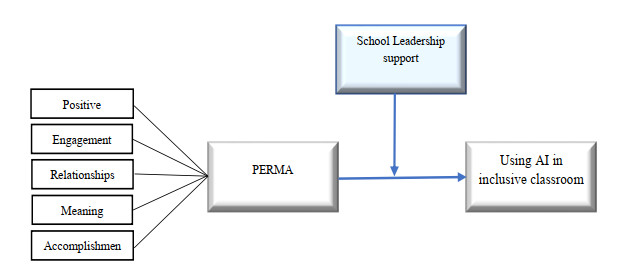
Integrating artificial intelligence (AI) into primary inclusive classrooms can significantly enhance teacher well-being by streamlining tasks, preventing burnout, fostering collaboration, and supporting diverse learning needs. However, for teachers to effectively use AI, they need to recognize its relevance, engage with its benefits, and promote its use to enhance their own well-being. The primary goal of this study is to examine the moderator effect of leadership support on the adoption of AI applications and tools and psychological well-being in primary inclusive classrooms in our hypothesized research model. To address this purpose, a quantitative methodology with structural equation modeling was utilized. Data was retrieved through an online questionnaire from 342 primary inclusive teachers, most being regular AI users. Our findings indicate that extensive use of AI tools is linked to engagement, relationships, and accomplishment but not to positive emotions or meaning. Surprisingly, school leadership negatively moderates factors outcomes, except for accomplishment, which remained effective. Leadership appeared less crucial in promoting AI adoption and enhancing teacher well-being. Leadership emerged as a less critical factor in promoting AI applications and tool adoption and teacher well-being. Professional programs for teachers should incorporate the impact of AI-based educational tools on psychological well-being, emphasizing the key role of leadership in AI adoption. Additionally, these programs should offer opportunities for sharing best practices to enhance the effective integration of AI in educational settings.

| [1] | Navarro-Espinosa, J.A., Vaquero-Abellán, M., Perea-Moreno, A.J., Pedrós-Pérez, G., Aparicio-Martínez, P. and Martínez-Jiménez, M.P., The influence of technology on mental well-being of stem teachers at university level: Covid-19 as a stressor. International journal of environmental research and public health, 2021, 18(18): 9605. |
| [2] | Thomas, L., Developing inclusive learning to improve the engagement, belonging, retention, and success of students from diverse groups. In Widening higher education participation, 2016,135‒159. Chandos Publishing. |
| [3] | Meidelina, O., Saleh, A.Y., Cathlin, C.A. and Winesa, S.A., Transformational Leadership and Teacher Well-Being: A Systematic Review. Journal of Education and Learning (EduLearn), 2023, 17(3): 417‒424. |
| [4] | Khansaheb, K.S.H.A., The Role of Artificial Intelligence in Enhancing Sustainability: The Case of UAE Smart Cities. BUiD Doctoral Research Conference 2023: Multidisciplinary Studies, 2024,235–242. https://doi.org/10.1007/978-3-031-56121-4_23 |
| [5] | Halder Adhya, D., Al Bastaki, E.M., Suleymanova, S., Muhammad, N. and Purushothaman, A., Utilizing open educational practices to support sustainable higher education in the United Arab Emirates. Asian Association of Open Universities Journal, 2024. https://doi.org/10.1108/AAOUJ-07-2023-0086 |
| [6] | Suresh, A., Jacobs, J., Clevenger, C., Lai, V., Tan, C., Martin, J.H., et al., Using AI to Promote Equitable Classroom Discussions: The TalkMoves Application. International conference on artificial intelligence in education, 2021,344–348. Cham: Springer International Publishing https://doi.org/10.1007/978-3-030-78270-2_61 |
| [7] |
Yao, Y., Wang, P., Jiang, Y., Li, Q. and Li, Y., Innovative online learning strategies for the successful construction of student self-awareness during the COVID-19 pandemic: Merging TAM with TPB. Journal of Innovation & Knowledge, 2022, 7(4): 100252. https://doi.org/10.1016/j.jik.2022.100252 doi: 10.1016/j.jik.2022.100252

|
| [8] | Huo, L. and Sun, F., Application of Artificial Intelligence in Mental Health Education in Primary and Middle Schools. Proceedings of the 2nd Conference on Artificial Intelligence and Healthcare, 2021,306–312. https://doi.org/10.5220/0011368000003444 |
| [9] | Luckin, R. and Holmes, W., Intelligence unleashed: An argument for ai in education, Pearson Education. 2016. |
| [10] |
Chua, K.H. and Bong, W.K., Providing inclusive education through virtual classrooms: a study of the experiences of secondary science teachers in Malaysia during the pandemic. International Journal of Inclusive Education, 2024, 28(9): 1886–1903. https://doi.org/10.1080/13603116.2022.2042403 doi: 10.1080/13603116.2022.2042403
|
| [11] |
Shamsuddinova, S., Heryani, P. and Naval, M.A., Evolution to revolution: Critical exploration of educators' perceptions of the impact of Artificial Intelligence (AI) on the teaching and learning process in the GCC region. International Journal of Educational Research, 2024,125: 102326. https://doi.org/10.1016/j.ijer.2024.102326 doi: 10.1016/j.ijer.2024.102326
|
| [12] |
Javed, A.R., Shahzad, F., ur Rehman, S., Zikria, Y.B., Razzak, I., Jalil, Z., et al., Future smart cities: requirements, emerging technologies, applications, challenges, and future aspects. Cities, 2022,129: 103794. https://doi.org/10.1016/j.cities.2022.103794 doi: 10.1016/j.cities.2022.103794
|
| [13] |
Jerrim, J. and Sims, S., When is high workload bad for teacher wellbeing? Accounting for the non-linear contribution of specific teaching tasks. Teaching and Teacher Education, 2021,105: 103395. https://doi.org/10.1016/j.tate.2021.103395 doi: 10.1016/j.tate.2021.103395
|
| [14] |
Karkouti, I.M., Abu-Shawish, R.K. and Romanowski, M.H., Teachers' understandings of the social and professional support needed to implement change in Qatar. Heliyon, 2022, 8(1): e08818. https://doi.org/10.1016/j.heliyon.2022.e08818 doi: 10.1016/j.heliyon.2022.e08818
|
| [15] | Flamholtz, E. and Randle, Y., Leading Strategic Change, Cambridge University Press, 2008. https://doi.org/10.1017/CBO9780511488528 |
| [16] | Skaalvik, E.M. and Skaalvik, S., Teacher Stress and Teacher Self-Efficacy: Relations and Consequences. In T. M. McIntyre, S. E. McIntyre, and D. J. Francis (Eds.), Educator Stress: An Occupational Health Perspective, 2017,101‒125. https://doi.org/10.1007/978-3-319-53053-6_5 |
| [17] |
Akiba, M., Byun, S., Jiang, X., Kim, K. and Moran, A.J., Do Teachers Feel Valued in Society? Occupational Value of the Teaching Profession in OECD Countries. AERA Open, 2023, 9: 23328584231179184. https://doi.org/10.1177/23328584231179184 doi: 10.1177/23328584231179184
|
| [18] | Hui, Z., Khan, N.A. and Akhtar, M., AI-based virtual assistant and transformational leadership in social cognitive theory perspective: a study of team innovation in construction industry. International Journal of Managing Projects in Business, 2024, 1‒20. |
| [19] |
Toropova, A., Myrberg, E. and Johansson, S., Teacher job satisfaction: the importance of school working conditions and teacher characteristics. Educational Review, 2021, 73(1): 71–97. https://doi.org/10.1080/00131911.2019.1705247 doi: 10.1080/00131911.2019.1705247
|
| [20] |
Heintzelman, S.J., Kushlev, K. and Diener, E, personalizing a positive psychology intervention improves well-being. Applied Psychology: Health and Well-Being, 2023, 15(4): 1271‒1292. https://doi.org/10.1111/aphw.12436 doi: 10.1111/aphw.12436
|
| [21] |
Guo, W., Li, W. and Tisdell, C.C., Effective pedagogy of guiding undergraduate engineering students solving first-order ordinary differential equations. Mathematics, 2021, 9(14): 1623. https://doi.org/10.3390/math9141623 doi: 10.3390/math9141623
|
| [22] |
Sun, R., Teulings, I. and Sauter, D., Why Being Social and Active Boosts Psychological Wellbeing: A Mediating Role of Momentary Positive Emotions. Social Psychological and Personality Science. 2023. https://doi.org/10.1177/19485506231218362 doi: 10.1177/19485506231218362
|
| [23] |
Xie, F. and Derakhshan, A., A Conceptual Review of Positive Teacher Interpersonal Communication Behaviors in the Instructional Context. Frontiers in Psychology, 2021, 12: 708490. https://doi.org/10.3389/fpsyg.2021.708490 doi: 10.3389/fpsyg.2021.708490
|
| [24] |
Billingsley, B., DeMatthews, D., Connally, K. and McLeskey, J., Leadership for Effective Inclusive Schools: Considerations for Preparation and Reform. Australasian Journal of Special and Inclusive Education, 2018, 42(01): 65–81. https://doi.org/10.1017/jsi.2018.6 doi: 10.1017/jsi.2018.6
|
| [25] |
Cann, R.F., Riedel-Prabhakar, R. and Powell, D., A Model of Positive School Leadership to Improve Teacher Wellbeing. International Journal of Applied Positive Psychology, 2021, 6(2): 195–218. https://doi.org/10.1007/s41042-020-00045-5 doi: 10.1007/s41042-020-00045-5
|
| [26] |
Du Plessis, A. and McDonagh, K., The out-of-field phenomenon and leadership for wellbeing: Understanding concerns for teachers, students and education partnerships. International Journal of Educational Research, 2021,106: 101724. https://doi.org/10.1016/j.ijer.2020.101724 doi: 10.1016/j.ijer.2020.101724
|
| [27] |
Nasir, M., Hasan, M., Adlim, A. and Syukri, M., Utilizing artificial intelligence in education to enhance teaching effectiveness. Proceedings of International Conference on Education, 2024, 2(1): 280–285. https://doi.org/10.32672/pice.v2i1.1367 doi: 10.32672/pice.v2i1.1367
|
| [28] | Sipahioglu, M., Empowering Teachers With Generative AI Tools and Support. Transforming Education With Generative AI: Prompt Engineering and Synthetic Content Creation, 2024,214–238. https://doi.org/10.4018/979-8-3693-1351-0.ch011 |
| [29] |
Thornton, K., Leading through COVID-19: New Zealand secondary principals describe their reality. Educational Management Administration & Leadership, 2021, 49(3): 393–409. https://doi.org/10.1177/1741143220985110 doi: 10.1177/1741143220985110
|
| [30] |
Kern, M.L., Waters, L., Adler, A. and White, M., Assessing Employee Wellbeing in Schools Using a Multifaceted Approach: Associations with Physical Health, Life Satisfaction, and Professional Thriving. Psychology, 2014, 5(6): 500–513. https://doi.org/10.4236/psych.2014.56060 doi: 10.4236/psych.2014.56060
|
| [31] |
Yeh, C.S.H. and Barrington, R., Sustainable positive psychology interventions enhance primary teachers' wellbeing and beyond – A qualitative case study in England. Teaching and Teacher Education, 2023,125: 104072. https://doi.org/10.1016/j.tate.2023.104072 doi: 10.1016/j.tate.2023.104072
|
| [32] |
Goetz, T., Botes, E., Resch, L.M., Weiss, S., Frenzel, A.C. and Ebner, M., Teachers emotionally profit from positive school leadership: Applying the PERMA-Lead model to the control-value theory of emotions. Teaching and Teacher Education, 2024,141: 104517. https://doi.org/10.1016/j.tate.2024.104517 doi: 10.1016/j.tate.2024.104517
|
| [33] |
Seligman, M., PERMA and the building blocks of well-being. The Journal of Positive Psychology, 2018, 13(4): 333–335. https://doi.org/10.1080/17439760.2018.1437466 doi: 10.1080/17439760.2018.1437466
|
| [34] | Burns, J.M., Leadership, NY: Harper & Row, 1978. |
| [35] |
Díaz, B. and Nussbaum, M., Artificial intelligence for teaching and learning in schools: The need for pedagogical intelligence. Computers & Education, 2024,217: 105071. https://doi.org/10.1016/j.compedu.2024.105071 doi: 10.1016/j.compedu.2024.105071
|
| [36] |
Popenici, S.A.D. and Kerr, S., Exploring the impact of artificial intelligence on teaching and learning in higher education. Research and Practice in Technology Enhanced Learning, 2017, 12(1): 22. https://doi.org/10.1186/s41039-017-0062-8 doi: 10.1186/s41039-017-0062-8
|
| [37] |
Su, J. and Yang, W., Artificial intelligence in early childhood education: A scoping review. Computers and Education: Artificial Intelligence, 2022, 3: 100049. https://doi.org/10.1016/j.caeai.2022.100049 doi: 10.1016/j.caeai.2022.100049
|
| [38] |
Ali, O., Murray, P.A., Momin, M., Dwivedi, Y.K. and Malik, T., The effects of artificial intelligence applications in educational settings: Challenges and strategies. Technological Forecasting and Social Change, 2024,199: 123076. https://doi.org/10.1016/j.techfore.2023.123076 doi: 10.1016/j.techfore.2023.123076
|
| [39] |
Ojha, A.K., Reflecting on management knowledge in India: Urgency to change the paradigm, decolonise and indigenise in the age of Artificial Intelligence. ⅡMB Management Review, 2024, 36(1): 7–20. https://doi.org/10.1016/j.iimb.2024.02.006 doi: 10.1016/j.iimb.2024.02.006
|
| [40] |
Adeleye, O.O., Eden, C.A. and Adeniyi, I.S., Innovative teaching methodologies in the era of artificial intelligence: A review of inclusive educational practices. World Journal of Advanced Engineering Technology and Sciences, 2024, 11(2): 069–079. https://doi.org/10.30574/wjaets.2024.11.2.0091 doi: 10.30574/wjaets.2024.11.2.0091
|
| [41] |
Ryan, R.M. and Deci, E.L., On Happiness and Human Potentials: A Review of Research on Hedonic and Eudaimonic Well-Being. Annual Review of Psychology, 2001, 52(1): 141–166. https://doi.org/10.1146/annurev.psych.52.1.141 doi: 10.1146/annurev.psych.52.1.141
|
| [42] |
Lester, L., Cefai, C., Cavioni, V., Barnes, A. and Cross, D., A Whole-School Approach to Promoting Staff Wellbeing. Australian Journal of Teacher Education, 2020, 45(2): 1–22. https://doi.org/10.14221/ajte.2020v45n2.1 doi: 10.14221/ajte.2020v45n2.1
|
| [43] | McLean, L. and Sandilos, L., Teachers' Well-Being: Sources, Implications, and Directions for Research. In Teachers' Well-Being: Sources, Implications, and Directions for Research, 2022. https://doi.org/10.4324/9781138609877-REE153-1 |
| [44] | Falecki, D. and Mann, E., Practical Applications for Building Teacher WellBeing in Education. Cultivating Teacher Resilience, 2021,175–191. Springer Singapore. https://doi.org/10.1007/978-981-15-5963-1_11 |
| [45] | O'Sullivan, C., Ryan, S. and O'Sullivan, L., Teacher Well-Being in Diverse School and Preschool Contexts. International perspectives on teacher well-being and diversity: Portals into innovative classroom practice, 2021,163–187. https://doi.org/10.1007/978-981-16-1699-0_8 |
| [46] |
Corcoran, R.P. and O'Flaherty, J., Social and emotional learning in teacher preparation: Pre-service teacher well-being. Teaching and Teacher Education, 2022,110: 103563. https://doi.org/10.1016/j.tate.2021.103563 doi: 10.1016/j.tate.2021.103563
|
| [47] |
Pearce, A., Achieving Academic Satisfaction through the use of Education-Based Technologies: Strengthening Students Personal Well-being While Facing Online Learning Mandates and Digital Disparities. Global Journal of Human-Social Science, 2021, 21(5): 19–36. https://doi.org/10.34257/LJRHSSVOL21IS5PG21 doi: 10.34257/LJRHSSVOL21IS5PG21
|
| [48] |
Cabrera, V. and Donaldson, S.I., PERMA to PERMA+4 building blocks of well-being: A systematic review of the empirical literature. The Journal of Positive Psychology, 2024, 19(3): 510–529. https://doi.org/10.1080/17439760.2023.2208099 doi: 10.1080/17439760.2023.2208099
|
| [49] |
Eloff, I. and Dittrich, A.K., Understanding general pedagogical knowledge influences on sustainable teacher well-being: A qualitative exploratory study. Journal of Psychology in Africa, 2021, 31(5): 464–469. https://doi.org/10.1080/14330237.2021.1978166 doi: 10.1080/14330237.2021.1978166
|
| [50] |
Ausat, A.M.A., Shafiq, M.A., Wafik, D. and López, N.A.S., The Role of Transformational Leadership in Improving Employee Psychological Wellbeing: A Review. Apollo: Journal of Tourism and Business, 2024, 2(1): 148–157. https://doi.org/10.58905/apollo.v2i1.239 doi: 10.58905/apollo.v2i1.239
|
| [51] |
Daniëls, E., Hondeghem, A. and Dochy, F., A review on leadership and leadership development in educational settings. Educational Research Review, 2019, 27: 110–125. https://doi.org/10.1016/j.edurev.2019.02.003 doi: 10.1016/j.edurev.2019.02.003
|
| [52] | Litz, D. and Blaik-Hourani, R., Transformational Leadership and Change in Education. In Oxford Research Encyclopedia of Education, Oxford University Press, 2020. https://doi.org/10.1093/acrefore/9780190264093.013.631 |
| [53] | Bass, B.M., From Transactional to Transformational Leadership: Learning to Share the Vision. In R. P. Vecchio (Ed.), Leadership: Understanding the Dynamics of Power and Influence in Organizations, Second Edition, 2007,302–317. University of Notre Dame Press. https://doi.org/10.2307/j.ctvpg85tk.29 |
| [54] |
McCarthy, A.M., Maor, D., McConney, A. and Cavanaugh, C., Digital transformation in education: Critical components for leaders of system change. Social Sciences & Humanities Open, 2023, 8(1): 100479. https://doi.org/10.1016/j.ssaho.2023.100479 doi: 10.1016/j.ssaho.2023.100479
|
| [55] |
Venema-Steen, I., Southall, A. and Bortoli, A., Drawing on the Locus of Control Framework to Explore the Role of School Leaders in Teacher Well-Being. Journal of Educational Research and Practice, 2023, 13(1). https://doi.org/10.5590/JERAP.2023.13.1.11 doi: 10.5590/JERAP.2023.13.1.11
|
| [56] | Voelkel, R.H., Supporting Effective Professional Learning Communities Through Developing Increased Principal Leadership Capacity. Proceedings of the 2022 AERA Annual Meeting. 2022. https://doi.org/10.3102/1890357 |
| [57] |
Cheng, E.C.K. and Wang, T., Leading digital transformation and eliminating barriers for teachers to incorporate artificial intelligence in basic education in Hong Kong. Computers and Education: Artificial Intelligence, 2023, 5: 100171. https://doi.org/10.1016/j.caeai.2023.100171 doi: 10.1016/j.caeai.2023.100171
|
| [58] |
Schmitz, M.L., Antonietti, C., Consoli, T., Cattaneo, A., Gonon, P. and Petko, D., Transformational leadership for technology integration in schools: Empowering teachers to use technology in a more demanding way. Computers & Education, 2023,204: 104880. https://doi.org/10.1016/j.compedu.2023.104880 doi: 10.1016/j.compedu.2023.104880
|
| [59] |
Raman, A., Don, Y. and Latif Kasim, A., The Relationship between Principals' Technology Leadership and Teachers' Technology Use in Malaysian Secondary Schools. Asian Social Science, 2014, 10(18): 30‒36. https://doi.org/10.5539/ass.v10n18p30 doi: 10.5539/ass.v10n18p30
|
| [60] |
Kern, M.L., Waters, L.E., Adler, A. and White, M.A., A multidimensional approach to measuring well-being in students: Application of the PERMA framework. The Journal of Positive Psychology, 2015, 10(3): 262–271. https://doi.org/10.1080/17439760.2014.936962 doi: 10.1080/17439760.2014.936962
|
| [61] |
Butler, J. and Kern, M.L., The PERMA-Profiler: A brief multidimensional measure of flourishing. International Journal of Wellbeing, 2016, 6(3): 1–48. https://doi.org/10.5502/ijw.v6i3.526 doi: 10.5502/ijw.v6i3.526
|
| [62] |
Mtebe, J.S., Mbwilo, B. and Kissaka, M.M., Factors Influencing Teachers' Use of Multimedia Enhanced Content in Secondary Schools in Tanzania. The International Review of Research in Open and Distributed Learning, 2016, 17(2): 65‒84. https://doi.org/10.19173/irrodl.v17i2.2280 doi: 10.19173/irrodl.v17i2.2280
|
| [63] |
Berkovich, I. and Eyal, O., Educational Leaders and Emotions. Review of Educational Research, 2015, 85(1): 129–167. https://doi.org/10.3102/0034654314550046 doi: 10.3102/0034654314550046
|
| [64] | Brown, T.A., Confirmatory factor analysis for applied research, Guilford publications, 2015. |
| [65] |
Hau, K.T. Book Review of Structural Equation Modeling With LISREL, PRELIS, and SIMPLIS: Basic Concepts, Applications, and Programming. Structural Equation Modeling: A Multidisciplinary Journal, 2000, 7(4): 640–643. https://doi.org/10.1207/S15328007SEM0704_8 doi: 10.1207/S15328007SEM0704_8
|
| [66] | Mercer, S., Oberdorfer, P. and Saleem, M., Helping Language Teachers to Thrive: Using Positive Psychology to Promote Teachers' Professional Well-Being, Positive psychology perspectives on foreign language learning and teaching, 2016,213–229. https://doi.org/10.1007/978-3-319-32954-3_12 |
| [67] |
Dreer, B., Teachers' well-being and job satisfaction: the important role of positive emotions in the workplace. Educational Studies, 2024, 50(1): 61–77. https://doi.org/10.1080/03055698.2021.1940872 doi: 10.1080/03055698.2021.1940872
|
| [68] |
Wassink, S.G., van Wingerden, J. and Poell, R.F., Correction: Meaningful work and resilience among teachers: The mediating role of work engagement and job crafting. PLOS ONE, 2022, 17(5): e0269347. https://doi.org/10.1371/journal.pone.0269347 doi: 10.1371/journal.pone.0269347
|
| [69] |
Polatcan, M., Özkan, P. and Bellibaş, M.Ş., Cultivating teacher innovativeness through transformational leadership and teacher agency in schools: the moderating role of teacher trust. Journal of Professional Capital and Community, 2024, 9(3): 227–242. https://doi.org/10.1108/JPCC-01-2024-0008 doi: 10.1108/JPCC-01-2024-0008
|
| [70] |
Brooks, M., Creely, E. and Laletas, S., Coping through the unknown: School staff wellbeing during the COVID-19 pandemic. International Journal of Educational Research Open, 2022, 3: 100146. https://doi.org/10.1016/j.ijedro.2022.100146 doi: 10.1016/j.ijedro.2022.100146
|
| [71] |
Orunbon, N.O. and Ibikunle, G.A., Principals' Toxic Leadership Behaviour and Teachers' Workplace Incivility in Public Senior Secondary Schools, Lagos State, Nigeria. EduLine: Journal of Education and Learning Innovation, 2023, 3(2): 202–213. https://doi.org/10.35877/454RI.eduline1717 doi: 10.35877/454RI.eduline1717
|
Figures(1) / Tables(6)
Samah Hatem Almaki, Nofouz Mafarja, Hamama Mubarak Saif Al Mansoori. Teacher well-being and use of artificial intelligence applications and tools: Moderation effects of leadership support in inclusive classroom[J]. STEM Education, 2025, 5(1): 109-129. doi: 10.3934/steme.2025006


 DownLoad: