Optimal synthesis of a planar mechanism using Matlab: Example of slider crank in a rowing motion

Med Amine LARIBI; Med Amine LARIBI

doi:10.3934/steme.2023001

STEM Education

2023, Volume 3, Issue 1: 1-14. doi: 10.3934/steme.2023001

Previous Article Next Article

Research article Special Issues

Optimal synthesis of a planar mechanism using Matlab: Example of slider crank in a rowing motion

Med Amine LARIBI ^,

Department of GMSC, Pprime Institute CNRS, ISAE-ENSMA, University of Poitiers, UPR 3346, France; med.amine.laribi@univ-poitiers.fr

Academic Editor: Mingfeng Wang

Received: 09 December 2022 Revised: 26 February 2023 Accepted: 07 March 2023 Published: 10 March 2023

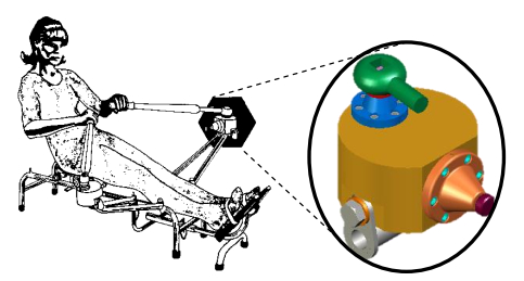
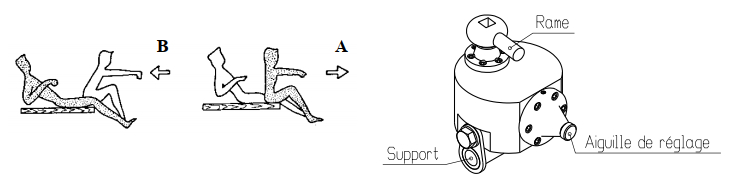
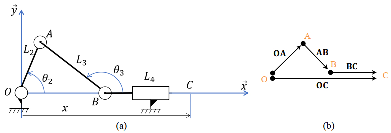
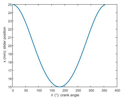
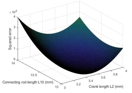
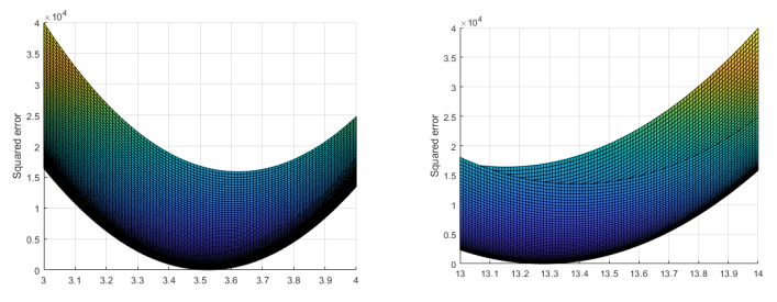
This paper illustrates the conducted effort to introduce the methodology of optimal synthesis of mechanisms through an engineering problem under Matlab. This project is part of a first course on poly-articulated mechanisms and robotics at the graduate level. The course combines both the theoretical and implementation under Matlab aspects to achieve its goals. The example of the rowing machine is considered to introduce the crank-slider mechanism and the kinematic analysis using complex numbers. The mechanism is associated with a spring to ensure the device simulating the resistance in the rowing bench simulator. The optimal synthesis problem is formulated for the desired effort to perform and solved using the Sequential Quadratic Programming method. All developments are implemented under Matlab.
- optimal synthesis,
- slider-crank,
- kinematic analysis,
- Matlab
Citation: Med Amine LARIBI. Optimal synthesis of a planar mechanism using Matlab: Example of slider crank in a rowing motion[J]. STEM Education, 2023, 3(1): 1-14. doi: 10.3934/steme.2023001

Related Papers:

Abstract

This paper illustrates the conducted effort to introduce the methodology of optimal synthesis of mechanisms through an engineering problem under Matlab. This project is part of a first course on poly-articulated mechanisms and robotics at the graduate level. The course combines both the theoretical and implementation under Matlab aspects to achieve its goals. The example of the rowing machine is considered to introduce the crank-slider mechanism and the kinematic analysis using complex numbers. The mechanism is associated with a spring to ensure the device simulating the resistance in the rowing bench simulator. The optimal synthesis problem is formulated for the desired effort to perform and solved using the Sequential Quadratic Programming method. All developments are implemented under Matlab.

References

[1]	Meriam, J.L. and Kraige, L.G., Engineering mechanics, Volume 2 Dynamics, Wiley, 1997.
[2]	Thibaut L., Ceuppens S., De Loof H., De Meester J., Goovaerts L., Struyf A., et al. (2018) Integrated STEM education: A systematic review of instructional practices in secondary education. European Journal of STEM Education 3: 2.
[3]	Ghani U., Zhai X., Ahmad R. (2021) Mathematics skills and STEM multidisciplinary literacy: Role of learning capacity. STEM Education 1: 104.
[4]	Koleza, E. and Skordoulis, C.D., Innovating STEM Education: Increased Engagement and Best Practices. Champaign, IL: Common Ground Research Networks. https://doi.org/10.18848/978-1-86335-251-2/CGP
[5]	Erdman, A.G. and Sandor, G.N., Mechanism Design: Analysis and Synthesis, 4th ed.; Pearson: London, UK, 2001.
[6]	Cabrera J., Simon A., Prado M. (2002) Optimal synthesis of mechanisms with genetic algorithms. Mech Mach Theory 37: 1165-1177.
[7]	Laribi M., Mlika A., Romdhane L., Zeghloul S. (2004) A combined genetic algorithm-fuzzy logic method GA-FL in mechanisms synthesis. Mech Mach Theory 39: 717-735.
[8]	McCarthy, J.M. and Joskowicz, L., Kinematic synthesis, Cambridge University Press, 2009.
[9]	Hernández A., Muñoyerro A., Urízar M., Amezua E. (2021) Comprehensive approach for the dimensional synthesis of a four-bar linkage based on path assessment and reformulating the error function. Mech Mach Theory 156: 104126.
[10]	Constans, E. and Dyer, K.B., Introduction to Mechanism Design with Computer Applications, CRC Press Taylor & Francis Group, 2019. https://doi.org/10.1201/b22145
[11]	Nocedal, J. and Wright, S., Numerical Optimization, Springer, 2006.

Author's biography Dr. Med Amine LARIBI is an Associate Professor in the Fundamental and Applied Sciences Faculty of the University of Poitiers (UP), where he teaches robotics and mechanic. He has a Mechanical Engineer Degree (specialization on Mechanical Design) from École Nationale d'Ingénieurs de Monsatir (E.N.I.M.) in 2001. M.S. in Mechanical Design, 2002. He received his Ph.D. in Mechanics from University of Poitiers in 2005 and National Habilitation in Mechanics from University of Poitiers in 2018. He servers as Associate Editor in several reputed internationals journals including ASME Journal of Medical Devices, Robotic Intelligence and Automation (Emerald Publishing), Mechanical Sciences (Copernicus Publications), MDPI Robotics and MDPI Machines. He is a member of international scientific committee of RAAD, MESROB and ROMANSY. His research interests, at the Department of G.M.S.C. of PPRIME Institute, include aspects on robots design, mechanism synthesis, cable driven robots, parallel robots, haptic interfaces, collaborative robots with more than 53 published peer reviewed journal papers, 9 edited books, 10 edited journal special issue, 6 PhD students. He is leading several national and international research projects in the fields of medical robotics and biomimetics

Reader Comments

Your name:*

Email:*
© 2023 the Author(s), licensee AIMS Press. This is an open access article distributed under the terms of the Creative Commons Attribution License (http://creativecommons.org/licenses/by/4.0)