Systematic review of mediterranean diet interventions in menopausal women

Carla Gonçalves; Helena Moreira; Ricardo Santos; Carla Gonçalves; Helena Moreira; Ricardo Santos

doi:10.3934/publichealth.2024005

AIMS Public Health

2024, Volume 11, Issue 1: 110-129. doi: 10.3934/publichealth.2024005

Previous Article Next Article

Review Special Issues

Systematic review of mediterranean diet interventions in menopausal women

1.
CITAB - Centre for the Research and Technology of Agro-Environmental and Biological Sciences, Institute for Innovation, Capacity Building and Sustainability of Agri-food Production (Inov4Agro), Universidade de Trás-os-Montes e Alto Douro, Vila Real, Portugal
2.
EPIUnit - Instituto de Saúde Pública - Laboratório para a Investigação Integrativa e Translacional em Saúde Populacional (ITR), Universidade do Porto, Porto, Portugal
3.
CISAS - Center for Research and Development in Agrifood Systems and Sustainability, Instituto Politécnico de Viana do Castelo, 4900-347 Viana do Castelo, Portugal
4.
CIDESD - Research Center in Sports Sciences, Health Sciences and Human Development, Laboratory of Biomechanics, Body Composition and Health (LaB2Health), Universidade de Trás-os-Montes e Alto Douro, Vila Real, Portugal
5.
CIFI2D - Centre of Research, Education, Innovation and Intervention in Sport, Faculdade de Desporto, Universidade do Porto, Porto, Portugal

Received: 20 September 2023 Revised: 21 December 2023 Accepted: 25 December 2023 Published: 10 January 2024

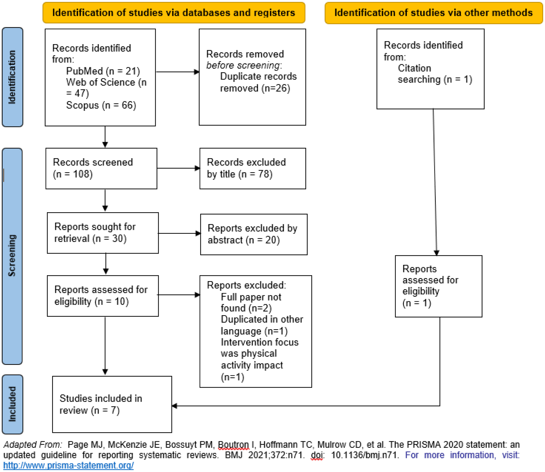
The increasing lifespan of women and their extended time spent in menopause pose significant challenges for health care systems, primarily due to the impacts of postmenopausal estrogen deficiency and aging on health. Menopause's onset is linked to a heightened prevalence of obesity, metabolic syndrome, cardiovascular disease, and osteoporosis. Diet is particularly relevant during menopause given its impact on quality of life and longevity and its modifiability. Because the Mediterranean diet is currently regarded as one of the healthiest dietary models in the world, the aim of this systematic review was to assess current evidence regarding the effectiveness of studies on the Mediterranean diet as an intervention for menopausal women. A systematic review of intervention-based studies involving the Mediterranean diet among menopausal women was performed in Scopus, PubMed, and Web of Science. The results of seven that met the inclusion criteria suggests that adherence to the Mediterranean diet can have beneficial impacts on menopausal women's health, including reductions in weight, blood pressure, blood ω6: ω3 ratio, triglycerides, total cholesterol, and LDL levels. Those results seem to be relevant for public health interventions aimed at improving menopausal women's quality of life.
- mediterranean diet,
- menopause,
- women's health,
- interventional studies
Citation: Carla Gonçalves, Helena Moreira, Ricardo Santos. Systematic review of mediterranean diet interventions in menopausal women[J]. AIMS Public Health, 2024, 11(1): 110-129. doi: 10.3934/publichealth.2024005

Related Papers:

Abstract

The increasing lifespan of women and their extended time spent in menopause pose significant challenges for health care systems, primarily due to the impacts of postmenopausal estrogen deficiency and aging on health. Menopause's onset is linked to a heightened prevalence of obesity, metabolic syndrome, cardiovascular disease, and osteoporosis. Diet is particularly relevant during menopause given its impact on quality of life and longevity and its modifiability. Because the Mediterranean diet is currently regarded as one of the healthiest dietary models in the world, the aim of this systematic review was to assess current evidence regarding the effectiveness of studies on the Mediterranean diet as an intervention for menopausal women. A systematic review of intervention-based studies involving the Mediterranean diet among menopausal women was performed in Scopus, PubMed, and Web of Science. The results of seven that met the inclusion criteria suggests that adherence to the Mediterranean diet can have beneficial impacts on menopausal women's health, including reductions in weight, blood pressure, blood ω6: ω3 ratio, triglycerides, total cholesterol, and LDL levels. Those results seem to be relevant for public health interventions aimed at improving menopausal women's quality of life.

Acknowledgments

This study is not funded by any agency and is being conducted by the authors independently. The authors CG and HM are researchers in CITAB, that is supported by FCT/UIDB/04033/2020. The author CG is researcher in EPIUnit, that is supported by FCT - Fundação para a Ciência e Tecnologia, I.P. through the projects with references UIDB/04750/2020 and LA/P/0064/2020 and DOI identifiers https://doi.org/10.54499/UIDB/04750/2020 and https://doi.org/10.54499/LA/P/0064/2020.

Conflict of Interest

The authors declare no conflict of interest.

References

[1]	Cavadas LF, Nunes A, Pinheiro M, et al. (2010) Management of menopause in primary health care. Acta Med Port 23: 227-236.
[2]	Ceylan B, Özerdoğan N (2015) Factors affecting age of onset of menopause and determination of quality of life in menopause. Turk J Obstet Gynecol 12: 43-49. https://doi.org/10.4274/tjod.79836
[3]	Nappi RE, Simoncini T (2021) Menopause transition: A golden age to prevent cardiovascular disease. Lancet Diabetes Endocrinol 9: 135-137. https://doi.org/10.1016/S2213-8587(21)00018-8
[4]	Silva TR, Oppermann K, Reis FM, et al. (2021) Nutrition in menopausal women: A narrative review. Nutrients 13: 2149. https://doi.org/10.3390/nu13072149
[5]	Di Daniele N, Noce A, Vidiri MF, et al. (2017) Impact of Mediterranean diet on metabolic syndrome, cancer and longevity. Oncotarget 8: 8947-8979. https://doi.org/10.18632/oncotarget.13553
[6]	Trichopoulou A, Costacou T, Bamia C, et al. (2003) Adherence to a Mediterranean diet and survival in a Greek population. N Engl J Med 348: 2599-2608. https://doi.org/10.1056/NEJMoa025039
[7]	Pes GM, Dore MP, Tsofliou F, et al. (2022) Diet and longevity in the Blue Zones: A set-and-forget issue?. Maturitas 164: 31-37. https://doi.org/10.1016/j.maturitas.2022.06.004
[8]	Morris L, Bhatnagar D (2016) The Mediterranean diet. Curr Opin Lipidol 27: 89-91. https://doi.org/10.1097/MOL.0000000000000266
[9]	Barbosa C, Real H, Pimenta P (2017) Roda da alimentação mediterrânica e pirâmide da dieta mediterrânica: comparação entre os dois guias alimentares. Acta Portuguesa de Nutrição 11: 6-14. https://doi.org/10.21011/apn.2017.1102
[10]	Castro-Quezada I, Román-Viñas B, Serra-Majem L (2014) The mediterranean diet and nutritional adequacy: A review. Nutrients 6: 231-248. https://doi.org/10.3390/nu6010231
[11]	Page MJ, Moher D, Bossuyt PM, et al. (2021) PRISMA 2020 explanation and elaboration: Updated guidance and exemplars for reporting systematic reviews. BMJ 372: n160. https://doi.org/10.1136/bmj.n160
[12]	Higgins JP, Savović J, Page MJ, et al. (2019) Assessing risk of bias in a randomized trial. Cochrane handbook for systematic reviews of interventions.Cureus 205-228. https://doi.org/10.1002/9781119536604.ch8
[13]	Sterne JA, Hernán MA, Reeves BC, et al. (2016) ROBINS-I: A tool for assessing risk of bias in non-randomised studies of interventions. BMJ 355: i4919. https://doi.org/10.1136/bmj.i4919
[14]	McGuinness LA, Higgins JPT (2021) Risk-of-bias VISualization (robvis): An R package and Shiny web app for visualizing risk-of-bias assessments. Res Synth Methods 12: 55-61. https://doi.org/10.1002/jrsm.1411
[15]	Rodriguez AS, Soidan JLG, Santos MDT, et al. (2016) Benefits of an educational intervention on diet and anthropometric profile of women with one cardiovascular risk factor. Medicina Clinica 146: 436-439. https://doi.org/10.1016/j.medcle.2016.06.047
[16]	Lombardo M, Perrone MA, Guseva E, et al. (2020) Losing weight after menopause with minimal aerobic training and mediterranean diet. Nutrients 12: 1-12. https://doi.org/10.3390/nu12082471
[17]	Vignini A, Nanetti L, Raffaelli F, et al. (2017) Effect of 1-y oral supplementation with vitaminized olive oil on platelets from healthy postmenopausal women. Nutrition 42: 92-98. https://doi.org/10.1016/j.nut.2017.06.013
[18]	Duś-Zuchowska M, Bajerska J, Krzyzanowska P, et al. (2018) The central European diet as an alternative to the mediterranean diet in atherosclerosis prevention in postmenopausal obese women with a high risk of metabolic syndrome-A randomized nutritional trial. Acta Sci Pol Technol Aliment 17: 399-407. https://doi.org/10.17306/J.AFS.0593
[19]	Muzsik A, Bajerska J, Jeleń HH, et al. (2019) FADS1 and FADS2 polymorphism are associated with changes in fatty acid concentrations after calorie-restricted Central European and Mediterranean diets. Menopause 26: 1415-1424. https://doi.org/10.1097/GME.0000000000001409
[20]	Bajerska J, Chmurzynska A, Muzsik A, et al. (2018) Weight loss and metabolic health effects from energy-restricted mediterranean and Central-European diets in postmenopausal women: A randomized controlled trial. Sci Rep 8: 11170. https://doi.org/10.1038/s41598-018-29495-3
[21]	Bihuniak JD, Ramos A, Huedo-Medina T, et al. (2016) Adherence to a mediterranean-style diet and its influence on cardiovascular risk factors in postmenopausal women. J Acad Nutr Diet 116: 1767-1775. https://doi.org/10.1016/j.jand.2016.06.377
[22]	Martínez-González MA, García-Arellano A, Toledo E, et al. (2012) A 14-item mediterranean diet assessment tool and obesity indexes among high-risk subjects: The PREDIMED trial. PLoS One 7: e43134. https://doi.org/10.1371/journal.pone.0043134
[23]	Panagiotakos DB, Pitsavos C, Stefanadis C (2006) Dietary patterns: A mediterranean diet score and its relation to clinical and biological markers of cardiovascular disease risk. Nutr Metab Cardiovasc Dis 16: 559-568. https://doi.org/10.1016/j.numecd.2005.08.006
[24]	Ganguly P, Alam SF (2015) Role of homocysteine in the development of cardiovascular disease. Nutr J 14: 1-10. https://doi.org/10.1186/1475-2891-14-6
[25]	Olén NB, Lehsten V (2022) High-resolution global population projections dataset developed with CMIP6 RCP and SSP scenarios for year 2010–2100. Data Brief 40: 107804. https://doi.org/10.1016/j.dib.2022.107804
[26]	Silva TRd, Martins CC, Ferreira LL, et al. (2019) Mediterranean diet is associated with bone mineral density and muscle mass in postmenopausal women. Climacteric 22: 162-168. https://doi.org/10.1080/13697137.2018.1529747
[27]	Al-Safi ZA, Polotsky AJ (2015) Obesity and menopause. Best Pract Res Clin Obstet Gynaecol 29: 548-553. https://doi.org/10.1016/j.bpobgyn.2014.12.002
[28]	Greendale GA, Sternfeld B, Huang M, et al. (2019) Changes in body composition and weight during the menopause transition. JCI Insight 4: e124865. https://doi.org/10.1172/jci.insight.124865
[29]	Maltais ML, Desroches J, Dionne IJ (2009) Changes in muscle mass and strength after menopause. J Musculoskelet Neuronal Interact 9: 186-197.
[30]	Aloia JF, McGowan DM, Vaswani AN, et al. (1991) Relationship of menopause to skeletal and muscle mass. Am J Clin Nutr 53: 1378-1383. https://doi.org/10.1093/ajcn/53.6.1378
[31]	Forsmo S, Hvam HM, Rea ML, et al. (2007) Height loss, forearm bone density and bone loss in menopausal women: a 15-year prospective study. The Nord-Trøndelag Health Study, Norway. Osteoporos Int 18: 1261-1269. https://doi.org/10.1007/s00198-007-0369-1
[32]	Mancini JG, Filion KB, Atallah R, et al. (2016) Systematic review of the Mediterranean diet for long-term weight loss. Am J Med 129: 407-415. https://doi.org/10.1016/j.amjmed.2015.11.028
[33]	Kim JY (2021) Optimal diet strategies for weight loss and weight loss maintenance. J Obes Metab Syndr 30: 20-31. https://doi.org/10.7570/jomes20065
[34]	Muscogiuri G, Verde L, Sulu C, et al. (2022) Mediterranean diet and obesity-related disorders: what is the evidence?. Curr Obes Rep 11: 287-304. https://doi.org/10.1007/s13679-022-00481-1
[35]	Dinu M, Pagliai G, Casini A, et al. (2018) Mediterranean diet and multiple health outcomes: An umbrella review of meta-analyses of observational studies and randomised trials. Eur J Clin Nutr 72: 30-43. https://doi.org/10.1038/ejcn.2017.58
[36]	Buckinx F, Aubertin-Leheudre M (2022) Sarcopenia in menopausal women: Current perspectives. Int J Womens Health 14: 805-819. https://doi.org/10.2147/IJWH.S340537
[37]	Finkelstein JS, Brockwell SE, Mehta V, et al. (2008) Bone mineral density changes during the menopause transition in a multiethnic cohort of women. J Clin Endocrinol Metab 93: 861-868. https://doi.org/10.1210/jc.2007-1876
[38]	Papadopoulou SK, Detopoulou P, Voulgaridou G, et al. (2023) Mediterranean diet and sarcopenia features in apparently healthy adults over 65 years: A systematic review. Nutrients 15: 1104. https://doi.org/10.3390/nu15051104
[39]	Antunes S, Marcelino O, Aguiar T (2003) Fisiopatologia da menopausa. Revista Portuguesa de Medicina Geral e Familiar 19: 353-357.
[40]	Taddei S (2009) Blood pressure through aging and menopause. Climacteric 12: 36-40. https://doi.org/10.1080/13697130903004758
[41]	Widmer RJ, Flammer AJ, Lerman LO, et al. (2015) The Mediterranean diet, its components, and cardiovascular disease. Am J Med 128: 229-238. https://doi.org/10.1016/j.amjmed.2014.10.014
[42]	Tuttolomondo A, Simonetta I, Daidone M, et al. (2019) Metabolic and vascular effect of the mediterranean diet. Int J Mol Sci 20: 4716. https://doi.org/10.3390/ijms20194716
[43]	Rizza S, Tesauro M, Cardillo C, et al. (2009) Fish oil supplementation improves endothelial function in normoglycemic offspring of patients with type 2 diabetes. Atherosclerosis 206: 569-574. https://doi.org/10.1016/j.atherosclerosis.2009.03.006
[44]	Paar M, Pavenstädt H, Kusche-Vihrog K, et al. (2014) Endothelial sodium channels trigger endothelial salt sensitivity with aging. Hypertension 64: 391-396. https://doi.org/10.1161/HYPERTENSIONAHA.114.03348
[45]	Viroli G, Gonçalves C, Pinho O, et al. (2021) High adherence to Mediterranean diet is not associated with an improved sodium and potassium intake. Nutrients 13: 4151. https://doi.org/10.3390/nu13114151
[46]	Goncalves C, Abreu S (2020) Sodium and potassium intake and cardiovascular disease in older people: A systematic review. Nutrients 12: 3447. https://doi.org/10.3390/nu12113447
[47]	Esposito K, Maiorino MI, Bellastella G, et al. (2015) A journey into a Mediterranean diet and type 2 diabetes: A systematic review with meta-analyses. BMJ Open 5: e008222. https://doi.org/10.1136/bmjopen-2015-008222
[48]	Sofi F, Cesari F, Abbate R, et al. (2008) Adherence to Mediterranean diet and health status: Meta-analysis. BMJ 337: a1344. https://doi.org/10.1136/bmj.a1344

publichealth-11-01-005-s001.pdf

Reader Comments

Your name:*

Email:*
© 2024 the Author(s), licensee AIMS Press. This is an open access article distributed under the terms of the Creative Commons Attribution License (http://creativecommons.org/licenses/by/4.0)