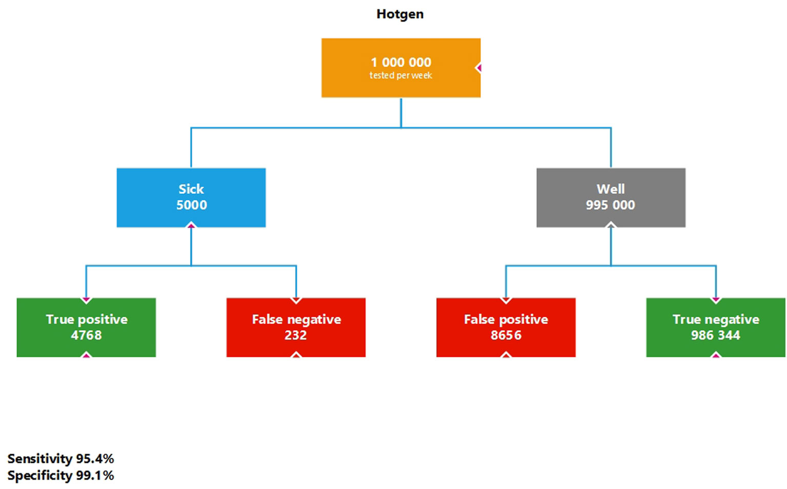
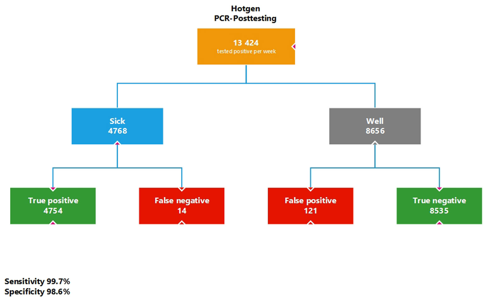
The aim of the current study is to perform model calculations on the possible use of SARS-CoV-2-rapid point-of-care tests as mass tests, using the quality criteria extracted from evidence-based research as an example for the Federal Republic of Germany. In addition to illustrating the problem of false positive test results, these calculations are used to examine their possible influence on the 7-day incidence. For a substantial period of time, this parameter formed the decisive basis for decisions on measures to protect the population in the wake of the COVID pandemic, which were taken by the government. Primarily, model calculations were performed for a base model of 1,000,000 SARS-CoV-2-rapid point-of-care tests per week using various sensitivities and specificities reported in the literature, followed by sequential testing of the test positives obtained by a SARS-CoV-2 PCR test. Furthermore, a calculation was performed for an actual maximum model based on self-test contingents by the German Federal Ministry of Health. Assuming a number of 1,000,000 tests per week at a prevalence of 0.5%, a high number of false positive test results, a low positive predictive value, a high negative predictive value, and an increase in the 7-day incidence due to the additional antigen rapid tests of approx. 5/100,000 were obtained. A previous maximum calculation based on contingent numbers for self-tests given by the German Federal Ministry of Health even showed an additional possible influence on the 7-day incidence of 84.6/100,000. The model calculations refer in each case to representative population samples that would have to be drawn if the successive results were comparable which should be given, as far-reaching actions were based on this parameter. The additionally performed SARS-CoV-2-rapid point-of-care tests increase the 7-day incidence in a clear way depending on the number of tests and clearly show their dependence on the respective number of tests. SARS-CoV-2-rapid point-of-care tests as well as the SARS-CoV-2-PCR test method should both be used exclusively in the presence of corresponding respiratory symptoms and not in symptom-free persons.
Citation: Oliver Hirsch, Werner Bergholz, Kai Kisielinski, Paul Giboni, Andreas Sönnichsen. Methodological problems of SARS-CoV-2 rapid point-of-care tests when used in mass testing[J]. AIMS Public Health, 2022, 9(1): 73-93. doi: 10.3934/publichealth.2022007
The aim of the current study is to perform model calculations on the possible use of SARS-CoV-2-rapid point-of-care tests as mass tests, using the quality criteria extracted from evidence-based research as an example for the Federal Republic of Germany. In addition to illustrating the problem of false positive test results, these calculations are used to examine their possible influence on the 7-day incidence. For a substantial period of time, this parameter formed the decisive basis for decisions on measures to protect the population in the wake of the COVID pandemic, which were taken by the government. Primarily, model calculations were performed for a base model of 1,000,000 SARS-CoV-2-rapid point-of-care tests per week using various sensitivities and specificities reported in the literature, followed by sequential testing of the test positives obtained by a SARS-CoV-2 PCR test. Furthermore, a calculation was performed for an actual maximum model based on self-test contingents by the German Federal Ministry of Health. Assuming a number of 1,000,000 tests per week at a prevalence of 0.5%, a high number of false positive test results, a low positive predictive value, a high negative predictive value, and an increase in the 7-day incidence due to the additional antigen rapid tests of approx. 5/100,000 were obtained. A previous maximum calculation based on contingent numbers for self-tests given by the German Federal Ministry of Health even showed an additional possible influence on the 7-day incidence of 84.6/100,000. The model calculations refer in each case to representative population samples that would have to be drawn if the successive results were comparable which should be given, as far-reaching actions were based on this parameter. The additionally performed SARS-CoV-2-rapid point-of-care tests increase the 7-day incidence in a clear way depending on the number of tests and clearly show their dependence on the respective number of tests. SARS-CoV-2-rapid point-of-care tests as well as the SARS-CoV-2-PCR test method should both be used exclusively in the presence of corresponding respiratory symptoms and not in symptom-free persons.

| [1] | Protzer U, Keppler O, Renz H, et al. Positionspapier des Netzwerk B-FAST im Nationalen Forschungsnetzwerk der Universitätsmedizin zu COVID-19 zur Anwendung und Zulassungspraxis von Antigen-Schnelltests zum Nachweis des neuen Coronavirus, SARS-CoV-2 (2021) .Available from: http://www.mvp.uni-muenchen.de/fileadmin/diagnostik/Teaserbilder/B-FAST_aktuell_Positionspapier_SARS-CoV-2-Ag-Schnelltests.pdf. |
| [2] | European Centre for Disease Prevention and Control (2020) Options for the use of rapid antigen tests for COVID-19 in the EU/EEA and the UK. Tech Rep . |
| [3] | Robert Koch Institut (RKI) Corona-Schnelltest-Ergebnisse verstehen, Berlin, 2021 Available from: https://www.rki.de/DE/Content/InfAZ/N/Neuartiges_Coronavirus/Infografik_Antigentest_PDF.pdf?__blob=publicationFile. |
| [4] | Dinnes J, Deeks JJ, Berhane S, et al. (2021) Rapid, point-of-care antigen and molecular-based tests for diagnosis of SARS-CoV-2 infection. Cochrane Database Syst Rev 3: CD013705. |
| [5] |
Riccò M, Ferraro P, Gualerzi G, et al. (2020) Point-of-care diagnostic tests for detecting SARS-CoV-2 antibodies: a systematic review and meta-analysis of real-world data. J Clin Med 9: 1515. doi: 10.3390/jcm9051515

|
| [6] | Robert Koch Institut (RKI) Epidemiologisches Bulletin, 2021 Available from: https://www.rki.de/DE/Content/Infekt/EpidBull/Archiv/2021/Ausgaben/03_21.pdf?__blob=publicationFile. |
| [7] |
Mina MJ, Peto TE, García-Fiñana M, et al. (2021) Clarifying the evidence on SARS-CoV-2 antigen rapid tests in public health responses to COVID-19. Lancet 397: 1425-1427. doi: 10.1016/S0140-6736(21)00425-6
|
| [8] | Corman VM, Landt O, Kaiser M, et al. (2020) Detection of 2019 novel coronavirus (2019-nCoV) by real-time RT-PCR. Euro Surveill 25: 2000045. |
| [9] | Zeichhardt H, Kammel M (2020) Kommentar zum Extra Ringversuch Gruppe 340 Virusgenom-Nachweis-SARS-CoV-2. Düsseldorf . |
| [10] |
Scohy A, Anantharajah A, Bodéus M, et al. (2020) Low performance of rapid antigen detection test as frontline testing for COVID-19 diagnosis. J Clin Virol 129: 104455. doi: 10.1016/j.jcv.2020.104455
|
| [11] |
Pray IW, Ford L, Cole D, et al. (2021) Performance of an antigen-based test for asymptomatic and symptomatic SARS-CoV-2 testing at two University campuses - Wisconsin, September-October 2020. MMWR Morb Mortal Wkly Rep 69: 1642-1647. doi: 10.15585/mmwr.mm695152a3
|
| [12] | Robert Koch Institut (RKI) Antworten auf häufig gestellte Fragen zum Coronavirus SARS-CoV-2/Krankheit COVID-19, 2021. Werden die Meldedaten durch die wachsende Anzahl an Schnelltests verzerrt? Available from: https://www.rki.de/SharedDocs/FAQ/NCOV2019/gesamt.html. |
| [13] | Salzberger B, Buder F, Lampl BT, et al. (2020) Epidemiologie von SARS-CoV-2/COVID-19. Gastroenterologe 1-7. |
| [14] | Schüller K Statistikerin: Positive Schnelltests sind meist falsch – selbst wenn sie Mediziner durchführen, 2021 Available from: https://www.focus.de/gesundheit/coronavirus/corona-infizierte-fruehzeitig-erkennen-statistikerin-positive-schnelltests-sind-meist-falsch-selbst-wenn-sie-medizin-personal-durchfuehrt_id_13061305.html. |
| [15] |
Pouwels KB, House T, Pritchard E, et al. (2021) Community prevalence of SARS-CoV-2 in England from April to November, 2020: results from the ONS Coronavirus Infection Survey. Lancet Public Health 6: e30-e38. doi: 10.1016/S2468-2667(20)30282-6
|
| [16] |
Vodičar PM, Oštrbenk Valenčak A, Zupan B, et al. (2020) Low prevalence of active COVID-19 in Slovenia: a nationwide population study of a probability-based sample. Clin Microbiol Infect 26: 1514-1519. doi: 10.1016/j.cmi.2020.07.013
|
| [17] |
Gudbjartsson DF, Helgason A, Jonsson H, et al. (2020) Spread of SARS-CoV-2 in the Icelandic population. N Engl J Med 382: 2302-2315. doi: 10.1056/NEJMoa2006100
|
| [18] | Snoeck CJ, Vaillant M, Abdelrahman T, et al. (2020) Prevalence of SARS-CoV-2 infection in the Luxembourgish population: the CON-VINCE study. medRxiv . |
| [19] | Robert Koch Institut (RKI) Täglicher Lagebericht des RKI zur Coronavirus-Krankheit-2019 (COVID-19), Berlin, 2021 Available from: https://www.rki.de/DE/Content/InfAZ/N/Neuartiges_Coronavirus/Situationsberichte/Maerz_2021/2021-03-31-de.pdf?__blob=publicationFile. |
| [20] | Bundesministerium für Gesundheit (German Ministry of Health) Fragen und Antworten zu Schnell- und Selbsttests zum Nachweis von SARS-CoV-2, 2021 Available from: https://www.bundesgesundheitsministerium.de/coronavirus/nationale-teststrategie/faq-schnelltests.html. |
| [21] | Statistisches Bundesamt Bevölkerungsstand, 2021 Available from: https://www.destatis.de/DE/Themen/Gesellschaft-Umwelt/Bevoelkerung/Bevoelkerungsstand/Tabellen/zensus-geschlecht-staatsangehoerigkeit-2020.html. |
| [22] | Grobbee DE, Hoes AW (2014) Clinical epidemiology: principles, methods, and applications for clinical research Jones&Bartlett Publishers. |
| [23] | World Health Organisation Recommendations for national SARS-CoV-2 testing strategies and diagnostic capacities. Interim guidance, Geneva, 2021 Available from: https://apps.who.int/iris/bitstream/handle/10665/342002/WHO-2019-nCoV-lab-testing-2021.1-eng.pdf?sequence=1&isAllowed=y. |
| [24] |
Cao S, Gan Y, Wang C, et al. (2020) Post-lockdown SARS-CoV-2 nucleic acid screening in nearly ten million residents of Wuhan, China. Nat Commun 11: 5917. doi: 10.1038/s41467-020-19802-w
|
| [25] |
Day M (2020) Covid-19: four fifths of cases are asymptomatic, China figures indicate. BMJ 369: m1375. doi: 10.1136/bmj.m1375
|
| [26] | Obi OC, Odoh DA (2021) Transmission of coronavirus (SARS-CoV-2) by presymptomatic and asymptomatic COVID-19 carriers: a systematic review. Eur J Med Educ Technol 1-7. |
| [27] |
Maniaci A, Iannella G, Vicini C, et al. (2020) A case of COVID-19 with late-onset rash and transient loss of taste and smell in a 15-year-old boy. Am J Case Rep 21: e925813. doi: 10.12659/AJCR.925813
|
| [28] |
Li DTS, Samaranayake LP, Leung YY, et al. (2021) Facial protection in the era of COVID-19: a narrative review. Oral Dis 27: 665-673. doi: 10.1111/odi.13460
|
| [29] |
Rothe C, Schunk M, Sothmann P, et al. (2020) Transmission of 2019-nCoV Infection from an asymptomatic contact in Germany. N Engl J Med 382: 970-971. doi: 10.1056/NEJMc2001468
|
| [30] |
Day M (2020) Covid-19: identifying and isolating asymptomatic people helped eliminate virus in Italian village. BMJ 368: m1165. doi: 10.1136/bmj.m1165
|
| [31] |
Lubrano R, Bloise S, Testa A, et al. (2021) Assessment of respiratory function in infants and young children wearing face masks during the COVID-19 pandemic. JAMA Netw Open 4: e210414. doi: 10.1001/jamanetworkopen.2021.0414
|
| [32] | Jefferson T, Spencer EA, Brassey J, et al. (2021) Transmission of severe acute respiratory syndrome coronavirus-2 (SARS-CoV-2) from pre and asymptomatic infected individuals. A systematic review. Clin Microbiol Infect S1198–743X(21)00616–9. |
| [33] | Savvides C, Siegel R (2020) Asymptomatic and presymptomatic transmission of SARS-CoV-2: a systematic review. medRxiv . |
| [34] |
Qiu X, Nergiz AI, Maraolo AE, et al. (2021) Defining the role of asymptomatic and pre-symptomatic SARS-CoV-2 transmission-a living systematic review. Clin Microbiol Infect 27: 511-519. doi: 10.1016/j.cmi.2021.01.011
|
| [35] | Seifried J, Böttcher S, Oh DY, et al. (2021) Was ist bei Antigentests zur Eigenanwendung (Selbsttests) zum Nachweis von SARS-CoV-2 zu beachten? Epidemiologisches Bull 8: 3-9. |
| [36] | World Health Organisation WHO Information Notice for IVD Users 2020/05. Nucleic acid testing (NAT) technologies that use polymerase chain reaction (PCR) for detection of SARS-CoV-2, 2021 Available from: https://www.who.int/news/item/20-01-2021-who-information-notice-for-ivd-users-2020-05. |
| [37] |
Strömer A, Rose R, Schäfer M, et al. (2020) Performance of a point-of-care test for the rapid detection of SARS-CoV-2 antigen. Microorganisms 9: 58. doi: 10.3390/microorganisms9010058
|
| [38] |
Iglὁi Z, Velzing J, van Beek J, et al. (2021) Clinical evaluation of Roche SD Biosensor rapid antigen test for SARS-CoV-2 in Municipal Health Service Testing Site, the Netherlands. Emerg Infect Dis 27: 1323-1329. doi: 10.3201/eid2705.204688
|
| [39] |
Bullard J, Dust K, Funk D, et al. (2020) Predicting infectious severe acute respiratory syndrome coronavirus 2 from diagnostic samples. Clin Infect Dis 71: 2663-2666. doi: 10.1093/cid/ciaa638
|
| [40] |
Stang A, Robers J, Schonert B, et al. (2021) The performance of the SARS-CoV-2 RT-PCR test as a tool for detecting SARS-CoV-2 infection in the population. J Infect 83: 244-245. doi: 10.1016/j.jinf.2021.05.022
|
| [41] |
Platten M, Hoffmann D, Grosser R, et al. (2021) SARS-CoV-2, CT-values, and infectivity-conclusions to be drawn from side observations. Viruses 13: 1459. doi: 10.3390/v13081459
|
| [42] | RWI – Leibniz-Institut für Wirtschaftsforschung Analysen zum Leistungsgeschehen der Krankenhäuser und zur Ausgleichspauschale in der Corona-Krise. Ergebnisse für den Zeitraum Januar bis Dezember 2020 Im Auftrag des Bundesministeriums für Gesundheit, Essen, 2021 Available from: https://www.bundesgesundheitsministerium.de/fileadmin/Dateien/3_Downloads/C/Coronavirus/Analyse_Leistungen_Ausgleichszahlungen_2020_Corona-Krise.pdf. |
| [43] |
Kowall B, Standl F, Oesterling F, et al. (2021) Excess mortality due to Covid-19? A comparison of total mortality in 2020 with total mortality in 2016 to 2019 in Germany, Sweden and Spain. PloS One 16: e0255540. doi: 10.1371/journal.pone.0255540
|
| [44] |
Arons MM, Hatfield KM, Reddy SC, et al. (2020) Presymptomatic SARS-CoV-2 infections and transmission in a skilled nursing facility. N Engl J Med 382: 2081-2090. doi: 10.1056/NEJMoa2008457
|
| [45] | Seifried J, Böttcher S, von Kleist M, et al. (2021) Antigentests als ergänzendes instrument in der Pandemiebekämpfung. Epidemiologisches Bull 17: 3-14. |
| [46] |
Kohn MA, Carpenter CR, Newman TB (2013) Understanding the direction of bias in studies of diagnostic test accuracy. Acad Emerg Med 20: 1194-1206. doi: 10.1111/acem.12255
|
| [47] |
Cheng HY, Jian SW, Liu DP, et al. (2020) Contact tracing assessment of COVID-19 transmission dynamics in Taiwan and risk at different exposure periods before and after symptom onset. JAMA Intern Med 180: 1156-1163. doi: 10.1001/jamainternmed.2020.2020
|
| [48] |
Madewell ZJ, Yang Y, Longini IM, et al. (2020) Household transmission of SARS-CoV-2: a systematic review and meta-analysis. JAMA Netw Open 3: e2031756. doi: 10.1001/jamanetworkopen.2020.31756
|
| [49] |
Gniazdowski V, Morris CP, Wohl S, et al. (2021) Repeat coronavirus disease 2019 molecular testing: correlation of SARS-CoV-2 culture with molecular assays and cycle thresholds. Clin Infect Dis 73: e860-e869. doi: 10.1093/cid/ciaa1616
|
| [50] |
Jefferson T, Spencer EA, Brassey J, et al. (2020) Viral cultures for COVID-19 infectious potential assessment - a systematic review. Clin Infect Dis ciaa1764. doi: 10.1093/cid/ciaa1764
|
| [51] |
Rao SN, Manissero D, Steele VR, et al. (2020) A systematic review of the clinical utility of cycle threshold values in the context of COVID-19. Infect Dis Ther 9: 573-586. doi: 10.1007/s40121-020-00324-3
|
| [52] |
Surkova E, Nikolayevskyy V, Drobniewski F (2020) False-positive COVID-19 results: hidden problems and costs. Lancet Respir Med 8: 1167-1168. doi: 10.1016/S2213-2600(20)30453-7
|
| [53] | Lühmann D (2020) Anlassloses Testen auf SARS-Cov-2. Für Personen, bei denen kein begründeter Verdacht auf eine Infektion vorliegt, ist die Aussagekraft eines einzelnen positiven Testergebnisses verschwindend gering. KVH J 9: 28-30. Available from: https://www.ebm-netzwerk.de/de/medien/pdf/ebm-9_20_kvh_journal_anlassloses-testen.pdf. |
| [54] | World Health Organisation Diagnostic testing for SARS-CoV-2. Interim guidance, Geneva, 2020 Available from: https://apps.who.int/iris/handle/10665/334254. |
| [55] |
Kohmer N, Toptan T, Pallas C, et al. (2021) The comparative clinical performance of four SARS-CoV-2 rapid antigen tests and their correlation to infectivity in vitro. J Clin Med 10: 328. doi: 10.3390/jcm10020328
|
| [56] |
Mboumba Bouassa RS, Veyer D, Péré H, et al. (2021) Analytical performances of the point-of-care SIENNA™ COVID-19 Antigen Rapid Test for the detection of SARS-CoV-2 nucleocapsid protein in nasopharyngeal swabs: a prospective evaluation during the COVID-19 second wave in France. Int J Infect Dis 106: 8-12. doi: 10.1016/j.ijid.2021.03.051
|
| [57] | Ioannidis JPA, Cripps S, Tanner MA (2020) Forecasting for COVID-19 has failed. Int J Forecast . |
| [58] |
Larremore DB, Wilder B, Lester E, et al. (2021) Test sensitivity is secondary to frequency and turnaround time for COVID-19 screening. Sci Adv 7: eabd5393. doi: 10.1126/sciadv.abd5393
|
| [59] |
Gelfand AE, Wang F (2000) Modelling the cumulative risk for a false-positive under repeated screening events. Stat Med 19: 1865-1879. doi: 10.1002/1097-0258(20000730)19:14<1865::AID-SIM512>3.0.CO;2-M
|
| [60] |
Thompson ML (2003) Assessing the diagnostic accuracy of a sequence of tests. Biostatistics 4: 341-351. doi: 10.1093/biostatistics/4.3.341
|
| [61] |
Iacobucci G (2021) Covid-19: mass testing at UK universities is haphazard and unscientific, finds BMJ investigation. BMJ 372: n848. doi: 10.1136/bmj.n848
|
| [62] | Ioannidis JPA (2021) Reconciling estimates of global spread and infection fatality rates of COVID-19: an overview of systematic evaluations. Eur J Clin Invest 51: e13554. |
 publichealth-09-01-007-s001.pdf publichealth-09-01-007-s001.pdf |
 |
| publichealth-09-01-007-s002.pdf |
|
Figures(4) / Tables(2)

Oliver Hirsch, Werner Bergholz, Kai Kisielinski, Paul Giboni, Andreas Sönnichsen. Methodological problems of SARS-CoV-2 rapid point-of-care tests when used in mass testing[J]. AIMS Public Health, 2022, 9(1): 73-93. doi: 10.3934/publichealth.2022007


 DownLoad: