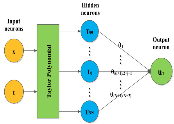
In this paper, the artificial neural network method is applied to solve the time-fractional diffusion and diffusion-wave equations. This method combines Taylor series and neural network method, and uses the terms of different power terms of Taylor series as neurons. An error function is given to update the weights of the proposed neural network. In addition, in order to balance the contributions of different error terms in the error function, we propose an adaptive weight adjustment method. In the end, four numerical examples are given to demonstrate the effectiveness of proposed method in solving the time-fractional diffusion and diffusion-wave equations.
Citation: Yinlin Ye, Hongtao Fan, Yajing Li, Ao Huang, Weiheng He. An artificial neural network approach for a class of time-fractional diffusion and diffusion-wave equations[J]. Networks and Heterogeneous Media, 2023, 18(3): 1083-1104. doi: 10.3934/nhm.2023047
In this paper, the artificial neural network method is applied to solve the time-fractional diffusion and diffusion-wave equations. This method combines Taylor series and neural network method, and uses the terms of different power terms of Taylor series as neurons. An error function is given to update the weights of the proposed neural network. In addition, in order to balance the contributions of different error terms in the error function, we propose an adaptive weight adjustment method. In the end, four numerical examples are given to demonstrate the effectiveness of proposed method in solving the time-fractional diffusion and diffusion-wave equations.

| [1] |
Y. A. Rossikhin, M. V. Shitikova, Applications of fractional calculus to dynamic problems of linear and nonlinear hereditary mechanics of solids, Appl. Mech. Rev., 50 (1997), 15–67. https://doi.org/10.1115/1.3101682 doi: 10.1115/1.3101682

|
| [2] |
D. del-Castillo-Negrete, B. A. Carreras, V. E. Lynch, Front dynamics in reaction-diffusion systems with Lévy flights: a fractional diffusion approach, Phys. Rev. Lett., 91 (2003), 018302. https://doi.org/10.1103/PhysRevLett.91.018302 doi: 10.1103/PhysRevLett.91.018302
|
| [3] |
A. Dechant, E. Lutz, Anomalous spatial diffusion and multifractality in optical lattices, Phys. Rev. Lett., 108 (2012), 230601. https://doi.org/10.1103/PhysRevLett.108.230601 doi: 10.1103/PhysRevLett.108.230601
|
| [4] |
M. Giona, H. E. Roman, Fractional diffusion equation for transport phenomena in random media, Phys. A, 185 (1992), 87–97. https://doi.org/10.1016/0378-4371(92)90441-R doi: 10.1016/0378-4371(92)90441-R
|
| [5] | F. Mainardi, Fractional diffusive waves in viscoelastic solids, In: J. I. Wegner, F. R. Norwood, eds., Nonlinear Waves in Solids., Fairfield: ASME/AMR, 1995, 93–97. |
| [6] |
W. H. Luo, T. Z. Huang, G. C. Wu, X. M. Gu, Quadratic spline collocation method for the time fractional subdiffusion equation, Appl. Math. Comput., 276 (2016), 252–265. https://doi.org/10.1016/j.amc.2015.12.020 doi: 10.1016/j.amc.2015.12.020
|
| [7] |
W. H. Luo, C. Li, T. Z. Huang, X. M. Gu, G. C. Wu, A high-order accurate numerical scheme for the Caputo derivative with applications to fractional diffusion problems, Numer. Funct. Anal. Optim., 39 (2018), 600–622. https://doi.org/10.1080/01630563.2017.1402346 doi: 10.1080/01630563.2017.1402346
|
| [8] |
X. M. Gu, S. L. Wu, A parallel-in-time iterative algorithm for Volterra partial integro-differential problems with weakly singular kernel, J. Comput. Phys., 417 (2020), 109576. https://doi.org/10.1016/j.jcp.2020.109576 doi: 10.1016/j.jcp.2020.109576
|
| [9] |
Y. L. Zhao, X. M. Gu, A. Ostermann, A preconditioning technique for an all-at-once system from Volterra subdiffusion equations with graded time steps, J. Sci. Comput., 88 (2021), 11. https://doi.org/10.1007/s10915-021-01527-7 doi: 10.1007/s10915-021-01527-7
|
| [10] |
Z. Liu, A. Cheng, X. Li, A novel finite difference discrete scheme for the time fractional diffusion-wave equation, Appl. Numer. Math., 134 (2018), 17–30. https://doi.org/10.1016/j.apnum.2018.07.001 doi: 10.1016/j.apnum.2018.07.001
|
| [11] |
R. Du, Y. Yan, Z. Liang, A high-order scheme to approximate the Caputo fractional derivative and its application to solve the fractional diffusion wave equation, J. Comput. Phys., 376 (2019), 1312–1330. https://doi.org/10.1016/j.jcp.2018.10.011 doi: 10.1016/j.jcp.2018.10.011
|
| [12] |
X. Li, S. Li, A fast element-free Galerkin method for the fractional diffusion-wave equation, Appl. Math. Lett., 122 (2021), 107529. https://doi.org/10.1016/j.aml.2021.107529 doi: 10.1016/j.aml.2021.107529
|
| [13] |
M. H. Heydari, M. R. Hooshmandasl, F. M. M. Ghaini, C. Cattani, Wavelets method for the time fractional diffusion-wave equation, Phys. Lett. A, 379 (2015), 71–76. https://doi.org/10.1016/j.physleta.2014.11.012 doi: 10.1016/j.physleta.2014.11.012
|
| [14] |
M. H. Heydari, Z. Avazzadeh, M. F. Haromi, A wavelet approach for solving multi-term variable-order time fractional diffusion-wave equation, Appl. Math. Comput., 341 (2019), 215–228. https://doi.org/10.1016/j.amc.2018.08.034 doi: 10.1016/j.amc.2018.08.034
|
| [15] |
A. Kumar, A. Bhardwaj, B. V. R. Kumar, A meshless local collocation method for time fractional diffusion wave equation, Comput. Math. Appl., 78 (2019), 1851–1861. https://doi.org/10.1016/j.camwa.2019.03.027 doi: 10.1016/j.camwa.2019.03.027
|
| [16] |
H. Qu, Cosine radial basis function neural networks for solving fractional differential equations, Adv. Appl. Math. Mech., 9 (2017), 667–679. https://doi.org/10.4208/aamm.2015.m909 doi: 10.4208/aamm.2015.m909
|
| [17] |
F. Rostami, A. Jafarian, A new artificial neural network structure for solving high-order linear fractional differential equations, Int. J. Comput. Math., 95 (2018), 528–539. https://doi.org/10.1080/00207160.2017.1291932 doi: 10.1080/00207160.2017.1291932
|
| [18] |
F. B. Rizaner, A. Rizaner, Approximate solutions of initial value problems for ordinary differential equations using radial basis function networks, Neural Process. Lett., 48 (2018), 1063–1071. https://doi.org/10.1007/s11063-017-9761-9 doi: 10.1007/s11063-017-9761-9
|
| [19] |
A. Jafarian, S. M. Nia, A. K. Golmankhaneh, B. Baleanu, On artificial neural networks approach with new cost functions, Appl. Math. Comput., 339 (2018), 546–555. https://doi.org/10.1016/j.amc.2018.07.053 doi: 10.1016/j.amc.2018.07.053
|
| [20] |
A. H. Hadian-Rasanan, D. Rahmati, S. Gorgin, K. Parand, A single layer fractional orthogonal neural network for solving various types of Lane-Emden equation, New Astron., 75 (2020), 101307. https://doi.org/10.1016/j.newast.2019.101307 doi: 10.1016/j.newast.2019.101307
|
| [21] |
H. Qu, X. Liu, Z. She, Neural network method for fractional-order partial differential equations, Neurocomputing, 414 (2020), 225–237. https://doi.org/10.1016/j.neucom.2020.07.063 doi: 10.1016/j.neucom.2020.07.063
|
| [22] |
Y. Ye, H. Fan, Y. Li, X. Liu, H. Zhang, Deep neural network methods for solving forward and inverse problems of time fractional diffusion equations with conformable derivative, Neurocomputing, 509 (2022), 177–192. https://doi.org/10.1016/j.neucom.2022.08.030 doi: 10.1016/j.neucom.2022.08.030
|
| [23] | A. A. Kilbas, H. M. Srivastava, J. J. Trujillo, Theory and Applications of Fractional Differential Equations, New York: Elsevier, 2006. |
| [24] | R. Garrappa, The Mittag-Leffler function, MATLAB Central File Exchange. Available from: https://www.mathworks.com/matlabcentral/fileexchange/48154-the-mittag-leffler-function |
| [25] | M. H. Hassoun, Fundamentals of artificial neural networks, Cambridge: MIT Press, 1995. |
| [26] | L. C. Evans, Partial Differential Equations, 2$^{nd}$ edition, Providence: American Mathematical Society, 2010. |
| [27] |
S. Wang, Y. Teng, P. Perdikaris, Understanding and mitigating gradient flow pathologies in physics-informed neural networks, SIAM J. Sci. Comput., 43 (2021), A3055–A3081. https://doi.org/10.1137/20M1318043 doi: 10.1137/20M1318043
|
| [28] |
J. Shen, X. M. Gu, Two finite difference methods based on an H2N2 interpolation for two-dimensional time fractional mixed diffusion and diffusion-wave equations, Discrete Contin. Dyn. Syst. Ser. B, 27 (2022), 1179–1207. https://doi.org/10.3934/dcdsb.2021086 doi: 10.3934/dcdsb.2021086
|
| [29] |
X. M. Gu, H. W. Sun, Y. L. Zhao, X. Zheng, An implicit difference scheme for time-fractional diffusion equations with a time-invariant type variable order, Appl. Math. Lett., 120 (2021), 107270. https://doi.org/10.1016/j.aml.2021.107270 doi: 10.1016/j.aml.2021.107270
|
| [30] |
X. M. Gu, T. Z. Huang, Y. L. Zhao, P. Lyu, B. Carpentieri, A fast implicit difference scheme for solving the generalized time-space fractional diffusion equations with variable coefficients, Numer Methods Partial Differ Equ, 37 (2021), 1136–1162. https://doi.org/10.1002/num.22571 doi: 10.1002/num.22571
|


Figures(9) / Tables(8)
Yinlin Ye, Hongtao Fan, Yajing Li, Ao Huang, Weiheng He. An artificial neural network approach for a class of time-fractional diffusion and diffusion-wave equations[J]. Networks and Heterogeneous Media, 2023, 18(3): 1083-1104. doi: 10.3934/nhm.2023047


 DownLoad: