We study continuum limits of discrete models for (possibly heterogeneous) nanowires. The lattice energy includes at least nearest and next-to-nearest neighbour interactions: the latter have the role of penalising changes of orientation. In the heterogeneous case, we obtain an estimate on the minimal energy spent to match different equilibria. This gives insight into the nucleation of dislocations in epitaxially grown heterostructured nanowires.
Citation: Roberto Alicandro, Giuliano Lazzaroni, Mariapia Palombaro. 2018: Derivation of a rod theory from lattice systems with interactions beyond nearest neighbours, Networks and Heterogeneous Media, 13(1): 1-26. doi: 10.3934/nhm.2018001
We study continuum limits of discrete models for (possibly heterogeneous) nanowires. The lattice energy includes at least nearest and next-to-nearest neighbour interactions: the latter have the role of penalising changes of orientation. In the heterogeneous case, we obtain an estimate on the minimal energy spent to match different equilibria. This gives insight into the nucleation of dislocations in epitaxially grown heterostructured nanowires.

| [1] |
Continuum limits of discrete thin films with superlinear growth densities. Calc. Var. Partial Differential Equations (2008) 33: 267-297. 
|
| [2] |
R. Alicandro, G. Lazzaroni and M. Palombaro, On the effect of interactions beyond nearest neighbours on non-convex lattice systems, Calc. Var. Partial Differential Equations, 56 (2017), Art. 42, 19 pp. |
| [3] |
L. Ambrosio, N. Fusco and D. Pallara, Functions of Bounded Variation and Free Discontinuity Problems, Oxford Mathematical Monographs, The Clarendon Press, Oxford University Press, New York, 2000. |
| [4] |
A. Braides, $Γ$ -convergence for Beginners, Oxford University Press, Oxford, 2002. |
| [5] |
Surface energies in nonconvex discrete systems. Math. Models Methods Appl. Sci. (2007) 17: 985-1037.
|
| [6] |
Asymptotic analysis of Lennard-Jones systems beyond the nearest-neighbour setting: A one-dimensional prototypical case. Math. Mech. Solids (2016) 21: 915-930.
|
| [7] |
Linear elastic chain with a hyper-pre-stress. J. Mech. Phys. Solids (2002) 50: 217-251.
|
| [8] |
G. Dal Maso, An Introduction to $Γ$ -convergence, Birkhäuser, Boston, 1993. |
| [9] |
E. Ertekin, P. A. Greaney, D. C. Chrzan and T. D. Sands, Equilibrium limits of coherency in strained nanowire heterostructures, J. Appl. Phys., 97 (2005), 114325. |
| [10] |
A variational model for dislocations at semi-coherent interfaces. J. Nonlinear Sci. (2017) 27: 1435-1461.
|
| [11] |
I. Fonseca, N. Fusco, G. Leoni and M. Morini, A model for dislocations in epitaxially strained elastic films, J. Math. Pures Appl., to appear (2018). |
| [12] |
A theorem on geometric rigidity and the derivation of nonlinear plate theory from three-dimensional elasticity. Comm. Pure Appl. Math. (2002) 55: 1461-1506.
|
| [13] |
K. L. Kavanagh, Misfit dislocations in nanowire heterostructures, Semicond. Sci. Technol., 25 (2010), 024006. |
| [14] |
A discrete to continuum analysis of dislocations in nanowire heterostructures. Commun. Math. Sci. (2015) 13: 1105-1133.
|
| [15] | Rigidity of three-dimensional lattices and dimension reduction in heterogeneous nanowires. Discrete Contin. Dyn. Syst. Ser. S (2017) 10: 119-139. |
| [16] | Derivation of a rod theory for multiphase materials. Calc. Var. Partial Differential Equations (2007) 28: 161-178. |
| [17] |
Derivation of a rod theory for biphase materials with dislocations at the interface. Calc. Var. Partial Differential Equations (2013) 48: 315-335.
|
| [18] |
On the passage from atomic to continuum theory for thin films. Arch. Ration. Mech. Anal. (2008) 190: 1-55.
|
| [19] |
Growth, thermodynamics, and electrical properties of silicon nanowires. Chem. Rev. (2010) 110: 361-388.
|
Figures(3)
Roberto Alicandro, Giuliano Lazzaroni, Mariapia Palombaro. 2018: Derivation of a rod theory from lattice systems with interactions beyond nearest neighbours, Networks and Heterogeneous Media, 13(1): 1-26. doi: 10.3934/nhm.2018001

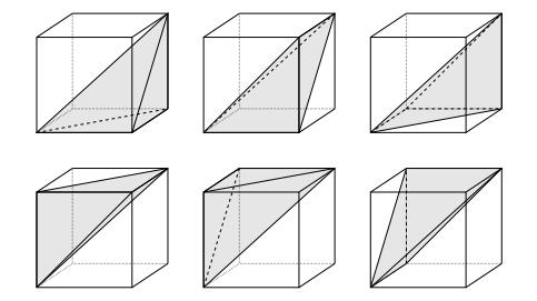
The six tetrahedra in the Kuhn decomposition of a three-dimensional cube
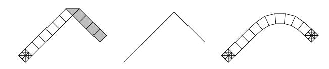
Two possible recovery sequences for the profile at the centre of the figure. Here we picture only a part of the wire containing just one species of atoms, therefore the transition at the interface is not represented. A kink in the profile may be reconstructed by folding the strip, i.e., mixing rotations and rotoreflections (left); or by a gradual transition involving only rotations or only rotoreflections (right). In the limit, the former recovery sequence gives a positive cost, while the latter gives no contribution. If the stronger topology is chosen, the appropriate recovery sequence will depend on the value of the internal variable, which defines the orientation of the wire
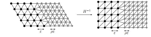
Lattices with dislocations: choice of the interfacial nearest neighbours in


 DownLoad: