Bayesian inference and impact of parameter prior specification in flexible multilevel nonlinear models in the context of infectious disease modeling

Olaiya Mathilde Adéoti; Aliou Diop; Romain Glèlè Kakaï; Olaiya Mathilde Adéoti; Aliou Diop; Romain Glèlè Kakaï

doi:10.3934/mbe.2025032

Mathematical Biosciences and Engineering

2025, Volume 22, Issue 4: 897-919. doi: 10.3934/mbe.2025032

Previous Article Next Article

Research article

Bayesian inference and impact of parameter prior specification in flexible multilevel nonlinear models in the context of infectious disease modeling

1.
Laboratoire de Biomathématiques et d'Estimations Forestières, University of Abomey-Calavi, Cotonou, Bénin
2.
Laboratoire d'Etude et de Recherche en Statistique et Developpement, Gaston Berger University, Saint-Louis Senegal

Academic Editor: Yang Kuang

Received: 27 December 2024 Revised: 23 February 2025 Accepted: 04 March 2025 Published: 07 March 2025

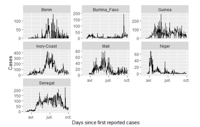
Bayesian flexible multilevel nonlinear models (FMNLMs) are powerful tools to analyze infectious disease data with asymmetric and unbalanced structures, such as varying epidemic stages across countries. However, the robustness of these models can be undermined by poorly designed estimation methods, particularly due to uncertainties in prior distributions and initial values. This study investigates how varying levels of prior informativeness can influence the model convergence, parameter estimation, and computation time in a Bayesian flexible multilevel nonlinear model (FMNLM). A simulation study was conducted to evaluate the impact of modifying prior assumptions on posterior estimates and their subsequent effects on the interpretations. The framework was applied to COVID-19 data from Francophone West Africa. The results indicate that accurate, informative priors enhance the prediction performance with minimal impact on the computation time. Conversely, non-informative or inaccurate priors for nonlinear parameters led to lower convergence rates and a reduced recovery accuracy, although they may remain viable in standard multilevel nonlinear models.
- nonlinear mixed models,
- infectious disease,
- sensitivity,
- epidemic dynamic,
- bayesian
Citation: Olaiya Mathilde Adéoti, Aliou Diop, Romain Glèlè Kakaï. Bayesian inference and impact of parameter prior specification in flexible multilevel nonlinear models in the context of infectious disease modeling[J]. Mathematical Biosciences and Engineering, 2025, 22(4): 897-919. doi: 10.3934/mbe.2025032

Related Papers:

Abstract

Bayesian flexible multilevel nonlinear models (FMNLMs) are powerful tools to analyze infectious disease data with asymmetric and unbalanced structures, such as varying epidemic stages across countries. However, the robustness of these models can be undermined by poorly designed estimation methods, particularly due to uncertainties in prior distributions and initial values. This study investigates how varying levels of prior informativeness can influence the model convergence, parameter estimation, and computation time in a Bayesian flexible multilevel nonlinear model (FMNLM). A simulation study was conducted to evaluate the impact of modifying prior assumptions on posterior estimates and their subsequent effects on the interpretations. The framework was applied to COVID-19 data from Francophone West Africa. The results indicate that accurate, informative priors enhance the prediction performance with minimal impact on the computation time. Conversely, non-informative or inaccurate priors for nonlinear parameters led to lower convergence rates and a reduced recovery accuracy, although they may remain viable in standard multilevel nonlinear models.

References

[1]	Y. Huang, D. Liu, H. Wu, Hierarchical bayesian methods for estimation of parameters in a longitudinal HIV dynamic system, Biometrics, 62 (2006), 413–423. https://doi.org/10.1111/j.1541-0420.2005.00447.x doi: 10.1111/j.1541-0420.2005.00447.x
[2]	Y. Huang, G. Dagne, Skew-normal bayesian nonlinear mixed-effects models with application to aids studies, Stat. Med., 29 (2010), 2384–2398. https://doi.org/10.1002/sim.3996 doi: 10.1002/sim.3996
[3]	S. Depaoli, The impact of inaccurate "informative" priors for growth parameters in bayesian growth mixture modeling, Struct. Equation Model. Multidiscip. J., 21 (2014), 239–252. https://doi.org/10.1080/10705511.2014.882686 doi: 10.1080/10705511.2014.882686
[4]	M. Kerioui, F. Mercier, J. Bertrand, C. Tardivon, R. Bruno, J. Guedj, et al., Bayesian inference using hamiltonian monte-carlo algorithm for nonlinear joint modeling in the context of cancer immunotherapy, Stat. Med., 39 (2020), 4853–4868. https://doi.org/10.1002/sim.8756 doi: 10.1002/sim.8756
[5]	M. D. Branco, D. K. Dey, A general class of multivariate skew-elliptical distributions, J. Multivar. Anal., 79 (2001), 99–113. https://doi.org/10.1006/jmva.2000.1960 doi: 10.1006/jmva.2000.1960
[6]	C. Meza, F. Osorio, R. De la Cruz, Estimation in nonlinear mixed-effects models using heavy-tailed distributions, Stat. Comput., 22 (2012), 121–139. https://doi.org/10.1007/s11222-010-9212-1 doi: 10.1007/s11222-010-9212-1
[7]	C. F. Tovissodé, A. Diop, R. Glèlè Kakaï, Inference in skew generalized t-link models for clustered binary outcome via a parameter-expanded EM algorithm, Plos One, 16 (2021), e0249604. https://doi.org/10.1371/journal.pone.0249604 doi: 10.1371/journal.pone.0249604
[8]	D. Zhang, M. Davidian, Linear mixed models with flexible distributions of random effects for longitudinal data, Biometrics, 57 (2001), 795–802. https://doi.org/10.1111/j.0006-341X.2001.00795.x doi: 10.1111/j.0006-341X.2001.00795.x
[9]	J. Chen, D. Zhang, M. Davidian, A Monte Carlo EM algorithm for generalized linear mixed models with flexible random effects distribution, Biostatistics, 3 (2002), 347–360. https://doi.org/10.1093/biostatistics/3.3.347 doi: 10.1093/biostatistics/3.3.347
[10]	E. Bonnet, O. Bodson, F. Le Marcis, A. Faye, N. Sambieni, F. Fournet, et al., The COVID-19 pandemic in Francophone West Africa: from the first cases to responses in seven countries, BMC Public Health, 21 (2021), 1–17. https://doi.org/10.1186/s12889-021-11529-7 doi: 10.1186/s12889-021-11529-7
[11]	E. Dong, H. Du, L. Gardner, An interactive web-based dashboard to track COVID-19 in real time, Lancet Infect. Dis., 20 (2020), 533–534.
[12]	V. H. Lachos, D. Bandyopadhyay, D. K. Dey, Linear and nonlinear mixed-effects models for censored HIV viral loads using normal/independent distributions, Biometrics, 67 (2011), 1594–1604. https://doi.org/10.1111/j.1541-0420.2011.01586.x doi: 10.1111/j.1541-0420.2011.01586.x
[13]	F. L. Schumacher, C. S. Ferreira, M. O. Prates, A. Lachos, V. H. Lachos, A robust nonlinear mixed-effects model for COVID-19 death data, Stat. Interface, 14 (2021), 49–57. https://doi.org/10.4310/20-SII637 doi: 10.4310/20-SII637
[14]	M. J. Lindstrom, D. M. Bates, Nonlinear mixed effects models for repeated measures data, Biometrics, (1990), 673–687. https://doi.org/10.2307/2532087 doi: 10.2307/2532087
[15]	V. H. Lachos, L. M. Castro, D. K. Dey, Bayesian inference in nonlinear mixed-effects models using normal independent distributions, Comput. Stat. Data Anal., 64 (2013), 237–252. https://doi.org/10.1016/j.csda.2013.02.011 doi: 10.1016/j.csda.2013.02.011
[16]	O. M. Adéoti, S. Agbla, A. Diop, R. G. Kakaï, Nonlinear mixed models and related approaches in infectious disease modeling: A systematic and critical review, Infect. Dis. Modell., 10 (2024), 110–128. https://doi.org/10.1016/j.idm.2024.09.001 doi: 10.1016/j.idm.2024.09.001
[17]	J. Chen, D. Zhang, M. Davidian, A Monte Carlo EM algorithm for generalized linear mixed models with flexible random effects distribution, Ph.D. thesis, Graduate Faculty of North Carolina State University, 2001.
[18]	M. Davidian, D. M. Giltinan, Nonlinear Models for Repeated Measurement Data, CRC press, 62 (1995).
[19]	M. Davidian, A. R. Gallant, The nonlinear mixed effects model with a smooth random effects density, Biometrika, 80 (1993), 475–488. https://doi.org/10.1093/biomet/80.3.475 doi: 10.1093/biomet/80.3.475
[20]	J. P. Hobert, G. Casella, The effect of improper priors on Gibbs sampling in hierarchical linear mixed models, J. Am. Stat. Assoc., 91 (1996), 1461–1473. https://doi.org/10.1080/01621459.1996.10476714 doi: 10.1080/01621459.1996.10476714
[21]	P. C. Bürkner, brms: An R package for bayesian multilevel models using Stan, J. Stat. Software, 80 (2017), 1–28. https://doi.org/10.18637/jss.v080.i01 doi: 10.18637/jss.v080.i01
[22]	T. Stan Development, Rstan: the r interface to stan, R packages 2.17.3. (2018).
[23]	R. C. Team, R: A language and environment for statistical computing (version 3.1. 2). vienna, austria. r foundation for statistical computing; 2014, 2019.
[24]	C. Team, Covidlp: short and long term prediction for COVID-19, Departamento de Estatıstica, UFMG, Brazil, 2020. Available from: http://est.ufmg.br/covidlp/home/en.
[25]	J. Wallinga, M. Lipsitch, How generation intervals shape the relationship between growth rates and reproductive numbers, Proc. R. Soc. B, 274 (2007), 599–604. https://doi.org/10.1098/rspb.2006.3754 doi: 10.1098/rspb.2006.3754
[26]	D. Makowski, M. S. Ben-Shachar, D. Lüdecke, bayestestR: Describing effects and their uncertainty, existence and significance within the bayesian framework, J. Open Source Software, 4 (2019), 1541. https://doi.org/10.21105/joss.01541 doi: 10.21105/joss.01541
[27]	J. M. Curran, An introduction to bayesian credible intervals for sampling error in DNA profiles, Law Probab. Risk, 4 (2005), 115–126. https://doi.org/10.1093/lpr/mgi009 doi: 10.1093/lpr/mgi009
[28]	S. H. Honfo, H. B. Taboe, R. G. Kakaï, Modeling COVID-19 dynamics in the sixteen West African countries, Sci. Afr., 18 (2022), e01408. https://doi.org/10.1016/j.sciaf.2022.e01408 doi: 10.1016/j.sciaf.2022.e01408
[29]	L. Tang, Y. Zhou, L. Wang, S. Purkayastha, L. Zhang, J. He, et al., A review of multi-compartment infectious disease models, Int. Stat. Rev., 88 (2020), 462–513. https://doi.org/10.1111/insr.12402 doi: 10.1111/insr.12402
[30]	J. E. Gnanvi, K. V. Salako, G. B. Kotanmi, R. Glèlè Kakaï, On the reliability of predictions on COVID-19 dynamics: A systematic and critical review of modelling techniques, Infect. Dis. Modell., 6 (2021), 258–272. https://doi.org/10.1016/j.idm.2020.12.008 doi: 10.1016/j.idm.2020.12.008
[31]	R. E. Kass, L. Wasserman, The selection of prior distributions by formal rules, J. Am. Stat. Assoc., 91 (1996), 1343–1370. https://doi.org/10.1080/01621459.1996.10477003 doi: 10.1080/01621459.1996.10477003
[32]	X. Tong, Z. Ke, Assessing the impact of precision parameter prior in bayesian non-parametric growth curve modeling, Front. Psychol., 12 (2021), 624588. https://doi.org/10.3389/fpsyg.2021.624588 doi: 10.3389/fpsyg.2021.624588
[33]	P. C. Lambert, A. J. Sutton, P. R. Burton, K. R. Abrams, D. R. Jones, How vague is vague? A simulation study of the impact of the use of vague prior distributions in MCMC using WinBUGS, Stat. Med., 24 (2005), 2401–2428. https://doi.org/10.1002/sim.2112 doi: 10.1002/sim.2112
[34]	Z. Zhang, F. Hamagami, L. Wang, J. R. Nesselroade, K. J. Grimm, Bayesian analysis of longitudinal data using growth curve models, Int. J. Behav. Dev., 31 (2007), 374–383. https://doi.org/10.1177/0165025407077764 doi: 10.1177/0165025407077764
[35]	R. Natarajan, C. E. McCulloch, Gibbs sampling with diffuse proper priors: A valid approach to data-driven inference?, J. Comput. Graphical Stat., 7 (1998), 267–277. https://doi.org/10.1080/10618600.1998.10474776 doi: 10.1080/10618600.1998.10474776

Reader Comments

Your name:*

Email:*
© 2025 the Author(s), licensee AIMS Press. This is an open access article distributed under the terms of the Creative Commons Attribution License (http://creativecommons.org/licenses/by/4.0)