Photovoltaic power prediction based on dilated causal convolutional network and stacked LSTM

Chongyi Tian; Longlong Lin; Yi Yan; Ruiqi Wang; Fan Wang; Qingqing Chi; Chongyi Tian; Longlong Lin; Yi Yan; Ruiqi Wang; Fan Wang; Qingqing Chi

doi:10.3934/mbe.2024049

Mathematical Biosciences and Engineering

2024, Volume 21, Issue 1: 1167-1185. doi: 10.3934/mbe.2024049

Previous Article Next Article

Research article Special Issues

Photovoltaic power prediction based on dilated causal convolutional network and stacked LSTM

1.
Shandong Key Laboratory of Intelligent Buildings Technology, School of Information and Electrical Engineering, Shandong Jianzhu University, Jinan 250101, China
2.
State Grid Shandong Integrated Energy Services CO., LTD, Jinan 250101, China

Academic Editor: Shangce Gao

Received: 08 September 2023 Revised: 12 November 2023 Accepted: 27 November 2023 Published: 25 December 2023

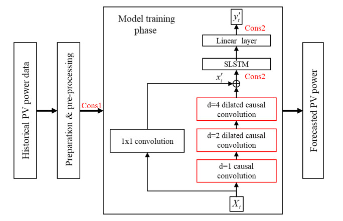
Due to the crucial role of photovoltaic power prediction in the integration, scheduling and operation of intelligent grid systems, the accuracy of prediction has garnered increasing attention from both the research and industry sectors. Addressing the challenges posed by the nonlinearity and inherent unpredictability of photovoltaic (PV) power generation sequences, this paper introduced a novel PV prediction model known as the dilated causal convolutional network and stacked long short-term memory (DSLSTM). The methodology begins by incorporating physical constraints to mitigate the limitations associated with machine learning algorithms, thereby ensuring that the predictions remain within reasonable bounds. Subsequently, a dilated causal convolutional network is employed to extract salient features from historical PV power generation data. Finally, the model adopts a stacked network structure to effectively enhance the prediction accuracy of the LSTM component. To validate the efficacy of the proposed model, comprehensive experiments were conducted using a real PV power generation dataset. These experiments involved comparing the predictive performance of the DSLSTM model against several popular existing models, including multilayer perceptron (MLP), recurrent neural network (RNN), long short-term memory (LSTM), gated recurrent unit (GRU), stacked LSTM and stacked GRU. Evaluation was performed using four key performance metrics: Mean absolute error (MAE), mean squared error (MSE), root mean squared error (RMSE) and R-squared (R2). The empirical results demonstrate that the DSLSTM model outperforms other models in terms of both prediction accuracy and stability.
- photovoltaic (PV) prediction,
- dilated causal convolution network (DCCN),
- stacked LSTM network,
- deep learning,
- hybrid deep learning
Citation: Chongyi Tian, Longlong Lin, Yi Yan, Ruiqi Wang, Fan Wang, Qingqing Chi. Photovoltaic power prediction based on dilated causal convolutional network and stacked LSTM[J]. Mathematical Biosciences and Engineering, 2024, 21(1): 1167-1185. doi: 10.3934/mbe.2024049

Related Papers:

Abstract

Due to the crucial role of photovoltaic power prediction in the integration, scheduling and operation of intelligent grid systems, the accuracy of prediction has garnered increasing attention from both the research and industry sectors. Addressing the challenges posed by the nonlinearity and inherent unpredictability of photovoltaic (PV) power generation sequences, this paper introduced a novel PV prediction model known as the dilated causal convolutional network and stacked long short-term memory (DSLSTM). The methodology begins by incorporating physical constraints to mitigate the limitations associated with machine learning algorithms, thereby ensuring that the predictions remain within reasonable bounds. Subsequently, a dilated causal convolutional network is employed to extract salient features from historical PV power generation data. Finally, the model adopts a stacked network structure to effectively enhance the prediction accuracy of the LSTM component. To validate the efficacy of the proposed model, comprehensive experiments were conducted using a real PV power generation dataset. These experiments involved comparing the predictive performance of the DSLSTM model against several popular existing models, including multilayer perceptron (MLP), recurrent neural network (RNN), long short-term memory (LSTM), gated recurrent unit (GRU), stacked LSTM and stacked GRU. Evaluation was performed using four key performance metrics: Mean absolute error (MAE), mean squared error (MSE), root mean squared error (RMSE) and R-squared (R2). The empirical results demonstrate that the DSLSTM model outperforms other models in terms of both prediction accuracy and stability.

References

[1]	Y. Dai, Y. Wang, M. Leng, X. Yang, Q. Zhou, LOWESS smoothing and random forest based GRU model: a short-term photovoltaic power generation forecasting method, Energy, 256 (2022), 124661. https://doi.org/10.1016/j.energy.2022.124661 doi: 10.1016/j.energy.2022.124661
[2]	H. Zhou, Y. Zhang, L. Yang, Q. Liu, K. Yan, Short-term photovoltaic power forecasting based on long short term memory neural network and attention mechanism, IEEE Access, 7 (2019), 78063–78074. https://doi.org/10.1109/ACCESS.2019.2923006 doi: 10.1109/ACCESS.2019.2923006
[3]	A. Khanlari, A. Sözen, C. Sirin, A. D. Tuncer, A. Gungor, Performance enhancement of a greenhouse dryer: analysis of a cost-effective alternative solar air heater, J. Clean. Prod., 251 (2020), 119672. https://doi.org/10.1016/j.jclepro.2019.119672 doi: 10.1016/j.jclepro.2019.119672
[4]	U. K. Das, K. S. Tey, S. Mehdi, S. Mekhilef, M. Y. I. Idris, W. Van Deventer, et al., Forecasting of photovoltaic power generation and model optimization: a review, Renew. Sustain. Energy Rev., 81 (2018), 912–928. https://doi.org/10.1016/j.rser.2017.08.017 doi: 10.1016/j.rser.2017.08.017
[5]	Y. Liu, Y. Liu, H. Cai, J. Zhang, An innovative short-term multihorizon photovoltaic power output forecasting method based on variational mode decomposition and a capsule convolutional neural network, Appl. Energy, 343 (2023), 121139. https://doi.org/10.1016/j.apenergy.2023.121139 doi: 10.1016/j.apenergy.2023.121139
[6]	S. Lin, C. Li, F. Xu, D. Liu, J. Liu, Risk identification and analysis for new energy power system in China based on d numbers and decision-making trial and evaluation laboratory (DEMATEL), J. Clean. Prod., 180 (2018), 81–96. https://doi.org /10.1016/j.jclepro.2018.01.153
[7]	R. Ahmed, V. Sreeram, Y. Mishra, M. D. Arif, A review and evaluation of the state-of-the-art in PV solar power forecasting: techniques and optimization, Renew. Sustain. Energy Rev., 124 (2020), 109792. https://doi.org/10.1016/j.rser.2020.109792 doi: 10.1016/j.rser.2020.109792
[8]	H. Wang, Y. Liu, B. Zhou, C. Li, G. Cao, N. Voropai, E. Barakhtenko, Taxonomy research of artificial intelligence for deterministic solar power forecasting, Energy Convers. Manage., 214 (2020), 112909. https://doi.org/10.1016/j.enconman.2020.112909 doi: 10.1016/j.enconman.2020.112909
[9]	A. Dolara, S. Leva, G. Manzolini, Comparison of different physical models for PV power output prediction, Sol. Energy, 119 (2015), 83–99. https://doi.org/10.1016/j.solener.2015.06.017 doi: 10.1016/j.solener.2015.06.017
[10]	D. Koster, F. Minette, C. Braun, O. Oliver, Short-term and regionalized photovoltaic power forecasting, enhanced by reference systems, on the example of Luxembourg, Renew. Energy, 132 (2019), 455–470. https://doi.org/10.1016/j.renene.2018.08.005 doi: 10.1016/j.renene.2018.08.005
[11]	F. Wang, Z. Zhen, C. Liu, Z. Mi, B. Hodge, M. Shafie-Khah, et al., Image phase shift invariance based cloud motion displacement vector calculation method for ultra-short-term solar PV power forecasting, Energy Convers. Manage., 157 (2018), 123–135. https://doi.org/10.1016/j.enconman.2017.11.080 doi: 10.1016/j.enconman.2017.11.080
[12]	H. Sharadga, S. Hajimirza, R. S. Balog, Time series forecasting of solar power generation for large-scale photovoltaic plants, Renew. Energy, 150 (2020), 797–807. https://doi.org/10.1016/j.renene.2019.12.131 doi: 10.1016/j.renene.2019.12.131
[13]	J. Müller, E. Trutnevyte, Spatial projections of solar PV installations at subnational level: accuracy testing of regression models, Appl. Energy, 265 (2020), 114747. https://doi.org/10.1016/j.apenergy.2020.114747 doi: 10.1016/j.apenergy.2020.114747
[14]	J. Boland, M. David, P. Lauret, Short term solar radiation forecasting: island versus continental sites, Energy, 113 (2016), 186–192. https://doi.org/10.1016/j.energy.2016.06.139 doi: 10.1016/j.energy.2016.06.139
[15]	M. Bouzerdoum, A. Mellit, A. Massi Pavan, A hybrid model (SARIMA–SVM) for short-term power forecasting of a small-scale grid-connected photovoltaic plant, Sol. Energy, 98 (2013), 226–235. https://doi.org/10.1016/j.solener.2013.10.002 doi: 10.1016/j.solener.2013.10.002
[16]	X. Luo, D. Zhang, X. Zhu, Deep learning based forecasting of photovoltaic power generation by incorporating domain knowledge, Energy, 225 (2021), 120240. https://doi.org/10.1016/j.energy.2021.120240 doi: 10.1016/j.energy.2021.120240
[17]	J. Liu, W. Fang, X. Zhang, C. Yang, An improved photovoltaic power forecasting model with the assistance of aerosol index data, IEEE T. Sustain. Energy, 6 (2015), 434–442. https://doi.org/10.1109/TSTE.2014.2381224 doi: 10.1109/TSTE.2014.2381224
[18]	M. Pan, C. Li, R. Gao, Y. Huang, H. You, T. Gu, et al., Photovoltaic power forecasting based on a support vector machine with improved ant colony optimization, J. Clean. Prod., 277 (2020), 123948. https://doi.org/10.1016/j.jclepro.2020.123948 doi: 10.1016/j.jclepro.2020.123948
[19]	P. Tang, D. Chen, Y. Hou, Entropy method combined with extreme learning machine method for the short-term photovoltaic power generation forecasting, Chaos Solitons Fractals, 89 (2016), 243–248. https://doi.org/10.1016/j.chaos.2015.11.008 doi: 10.1016/j.chaos.2015.11.008
[20]	Y. Ju, J. Li, G. Sun, Ultra-short-term photovoltaic power prediction based on self-attention mechanism and multi-task learning, IEEE Access, 8 (2020), 44821–44829. https://doi.org/10.1109/ACCESS.2020.2978635 doi: 10.1109/ACCESS.2020.2978635
[21]	X. Qing, Y. Niu, Hourly day-ahead solar irradiance prediction using weather forecasts by LSTM, Energy, 148 (2018), 461–468. https://doi.org/10.1016/j.energy.2018.01.177 doi: 10.1016/j.energy.2018.01.177
[22]	X. Guo, Y. Mo, K. Yan, Short-term photovoltaic power forecasting based on historical information and deep learning methods, Sensors, 22 (2022). https://doi.org/10.3390/s22249630 doi: 10.3390/s22249630
[23]	Y. He, Q. Gao, Y. Jin, F. Liu, Short-term photovoltaic power forecasting method based on convolutional neural network, Energy Rep., 8 (2022), 54–62. https://doi.org/10.1016/j.egyr.2022.10.071 doi: 10.1016/j.egyr.2022.10.071
[24]	S. Bai, J.Z. Kolter, V. Koltun, An empirical evaluation of generic convolutional and recurrent networks for sequence modeling, preprint, arXiv: 1803.01271.
[25]	S. Hochreiter, J. Schmidhuber, Long short-term memory, Neural Comput., 9 (1997), 1735–1780. https://doi.org/10.1162/neco.1997.9.8.1735 doi: 10.1162/neco.1997.9.8.1735
[26]	A. Ajami, M. Daneshvar, Data driven approach for fault detection and diagnosis of turbine in thermal power plant using independent component analysis (ICA), Int. J. Electr. Power Energy Syst., 43 (2012), 728–735. https://doi.org/10.1016/j.ijepes.2012.06.022 doi: 10.1016/j.ijepes.2012.06.022
[27]	J. Li, F. Guo, A. Sivakumar, Y. Dong, R. Krishnan, Transferability improvement in short-term traffic prediction using stacked LSTM network, Trans. Res. Emerging Technol., 124 (2021), 102977. https://doi.org/10.1016/j.trc.2021.102977 doi: 10.1016/j.trc.2021.102977
[28]	Z. Fazlipour, E. Mashhour, M. Joorabian, A deep model for short-term load forecasting applying a stacked autoencoder based on LSTM supported by a multi-stage attention mechanism, Appl. Energy, 327 (2022), 120063. https://doi.org/10.1016/j.apenergy.2022.120063 doi: 10.1016/j.apenergy.2022.120063

Reader Comments

Your name:*

Email:*
© 2024 the Author(s), licensee AIMS Press. This is an open access article distributed under the terms of the Creative Commons Attribution License (http://creativecommons.org/licenses/by/4.0)