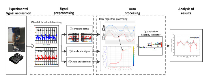
In this study, an accurate tool is provided for the evaluation of the effect of joint motion effect on gait stability. This quantitative gait evaluation method relies exclusively on the analysis of data acquired using acceleration sensors. First, the acceleration signal of lower limb motion is collected dynamically in real-time through the acceleration sensor. Second, an algorithm based on improved dynamic time warping (DTW) is proposed and used to calculate the gait stability index of the lower limbs. Finally, the effects of different joint braces on gait stability are analyzed. The experimental results show that the joint brace at the ankle and the knee reduces the range of motions of both ankle and knee joints, and a certain impact is exerted on the gait stability. In comparison to the ankle joint brace, the knee joint brace inflicts increased disturbance on the gait stability. Compared to the joint motion of the braced side, which showed a large deviation, the joint motion of the unbraced side was more similar to that of the normal walking process. In this paper, the quantitative evaluation algorithm based on DTW makes the results more intuitive and has potential application value in the evaluation of lower limb dysfunction, clinical training and rehabilitation.
Citation: Xuecheng Weng, Chang Mei, Farong Gao, Xudong Wu, Qizhong Zhang, Guangyu Liu. A gait stability evaluation method based on wearable acceleration sensors[J]. Mathematical Biosciences and Engineering, 2023, 20(11): 20002-20024. doi: 10.3934/mbe.2023886
In this study, an accurate tool is provided for the evaluation of the effect of joint motion effect on gait stability. This quantitative gait evaluation method relies exclusively on the analysis of data acquired using acceleration sensors. First, the acceleration signal of lower limb motion is collected dynamically in real-time through the acceleration sensor. Second, an algorithm based on improved dynamic time warping (DTW) is proposed and used to calculate the gait stability index of the lower limbs. Finally, the effects of different joint braces on gait stability are analyzed. The experimental results show that the joint brace at the ankle and the knee reduces the range of motions of both ankle and knee joints, and a certain impact is exerted on the gait stability. In comparison to the ankle joint brace, the knee joint brace inflicts increased disturbance on the gait stability. Compared to the joint motion of the braced side, which showed a large deviation, the joint motion of the unbraced side was more similar to that of the normal walking process. In this paper, the quantitative evaluation algorithm based on DTW makes the results more intuitive and has potential application value in the evaluation of lower limb dysfunction, clinical training and rehabilitation.

| [1] |
G. M. Scalera, M. Ferrarin, M. Rabuffetti, Gait regularity assessed by wearable sensors: Comparison between accelerometer and gyroscope data for different sensor locations and walking speeds in healthy subjects, J. Biomech., 113 (2020), 110115. https://doi.org/10.1016/j.jbiomech.2020.110115 doi: 10.1016/j.jbiomech.2020.110115

|
| [2] |
Y. P. Demir, S. A. Yildirim, Different walk aids on gait parameters and kinematic analysis of the pelvis in patients with adult neuromuscular disease, Neurosciences, 24 (2019), 36–44. https://doi.org/10.17712/nsj.2019.1.20180316 doi: 10.17712/nsj.2019.1.20180316
|
| [3] |
Y. Wang, Z. Liu, J. Xu, W. Yan, Heterogeneous network representation learning approach for ethereum identity identification, IEEE Trans. Comput. Soc. Syst., 10 (2023), 890–899. https://doi.org/10.1109/TCSS.2022.3164719 doi: 10.1109/TCSS.2022.3164719
|
| [4] |
K. G. M. Quispe, W. S. Lima, D. M. Batista, E. Souto, MBOSS: A symbolic representation of human activity recognition using mobile sensors, Sensors, 18 (2018). https://doi.org/10.3390/s18124354 doi: 10.3390/s18124354
|
| [5] |
S. Bahadori, J. M. Williams, T. W. Wainwright, Lower limb kinematic, kinetic and spatial-temporal gait data for healthy adults using a self-paced treadmill, Data Brief, 34 (2021), 106613. https://doi.org/10.1016/j.dib.2020.106613 doi: 10.1016/j.dib.2020.106613
|
| [6] |
M. F. Antwi-Afari, H. Li, Fall risk assessment of construction workers based on biomechanical gait stability parameters using wearable insole pressure system, Adv. Eng. Inf., 38 (2018), 683–694. https://doi.org/10.1016/j.aei.2018.10.002 doi: 10.1016/j.aei.2018.10.002
|
| [7] |
H. Ohtsu, S. Yoshida, T. Minamisawa, N. Katagiri, T. Yamaguchi, T. Takahashi, et al., Does the balance strategy during walking in elderly persons show an association with fall risk assessment?, J. Biomech., 103 (2020), 109657. https://doi.org/10.1016/j.jbiomech.2020.109657 doi: 10.1016/j.jbiomech.2020.109657
|
| [8] |
J. R. Brickner, J. L. Garzon, K. A. Cimprich, Walking a tightrope: The complex balancing act of R-loops in genome stability, Mol. Cell, 82 (2022), 2267–2297. https://doi.org/10.1016/j.molcel.2022.04.014 doi: 10.1016/j.molcel.2022.04.014
|
| [9] |
J. C. Schrijvers, J. C. van den Noort, M. van der Esch, J. Dekker, J. Harlaar, Objective parameters to measure (in)stability of the knee joint during gait: A review of literature, Gait Posture, 70 (2019), 235–253. https://doi.org/10.1016/j.gaitpost.2019.03.016 doi: 10.1016/j.gaitpost.2019.03.016
|
| [10] |
J. N. Katz, K. R. Arant, R. F. Loeser, Diagnosis and treatment of hip and knee osteoarthritis: A Review, J. Am. Med. Assoc., 325 (2021), 568–578. https://doi.org/10.1001/jama.2020.22171 doi: 10.1001/jama.2020.22171
|
| [11] |
M. Wang, X. Wang, C. Peng, S. Zhang, Z. Fan, Z. Liu, Research on EMG segmentation algorithm and walking analysis based on signal envelope and integral electrical signal, Photonic Netwrk Commun., 37 (2019), 195–203. https://doi.org/10.1007/s11107-018-0809-1 doi: 10.1007/s11107-018-0809-1
|
| [12] |
S. Borel, P. Schneider, C. J. Newman, Video analysis software increases the interrater reliability of video gait assessments in children with cerebral palsy, Gait Posture, 33 (2011), 727–729. https://doi.org/10.1016/j.gaitpost.2011.02.012 doi: 10.1016/j.gaitpost.2011.02.012
|
| [13] |
S. Chakraborty, A. Nandy, T. Yamaguchi, V. Bonnet, G. Venture, Accuracy of image data stream of a markerless motion capture system in determining the local dynamic stability and joint kinematics of human gait, J. Biomech., 104 (2020), 109718. https://doi.org/10.1016/j.gaitpost.2011.02.012 doi: 10.1016/j.gaitpost.2011.02.012
|
| [14] |
C. N. Armitano, H. J. Bennett, J. A. Haegele, S. Morrison, Assessment of the gait-related acceleration patterns in adults with autism spectrum disorder, Gait Posture, 75 (2020), 155–162. https://doi.org/10.1016/j.gaitpost.2019.09.002 doi: 10.1016/j.gaitpost.2019.09.002
|
| [15] |
Y. Shi, H. Li, X. Fu, R. Luan, Y. Wang, N. Wang, et al., Self-powered difunctional sensors based on sliding contact-electrification and tribovoltaic effects for pneumatic monitoring and controlling, Nano Energy, 110 (2023), 108339. https://doi.org/10.1016/j.nanoen.2023.108339 doi: 10.1016/j.nanoen.2023.108339
|
| [16] |
C. Mei, F. Gao, Y. Li, A determination method for gait event based on acceleration sensors, Sensors, 19 (2019), 5499. https://doi.org/10.3390/s19245499 doi: 10.3390/s19245499
|
| [17] |
J. Taborri, E. Palermo, S. Rossi, P. Cappa, Gait partitioning methods: A systematic review, Sensors, 16 (2016), 66. https://doi.org/10.3390/s16010066 doi: 10.3390/s16010066
|
| [18] | H. Chen, F. Gao, C. Chen, T. Tian, Estimation of ankle angle based on multi-feature fusion with random forest, in 2018 37th Chinese Control Conference (CCC), IEEE, (2018), 5549–5553. |
| [19] |
M. D. Gor-García-Fogeda, R. Cano de la Cuerda, M. Carratalá Tejada, I. M. Alguacil-Diego, F. Molina-Rueda, Observational gait assessments in people with neurological disorders: A systematic review, Arch. Phys. Med. Rehabil., 97 (2016), 131–140. https://doi.org/10.1016/j.apmr.2015.07.018 doi: 10.1016/j.apmr.2015.07.018
|
| [20] |
C. R. Brown, S. J. Hillman, A. M. Richardson, J. L. Herman, J. E. Robb, Reliability and validity of the visual gait assessment scale for children with hemiplegic cerebral palsy when used by experienced and inexperienced observers, Gait Posture, 27 (2008), 648–652. https://doi.org/10.1016/j.gaitpost.2007.08.008 doi: 10.1016/j.gaitpost.2007.08.008
|
| [21] |
C. H. Lee, S. H. Chen, B. C. Jiang, T. L. Sun, Estimating postural stability using improved permutation entropy via tug accelerometer data for community-dwelling elderly people, Entropy, 22 (2020), 354–365. https://doi.org/10.3390/e22101097 doi: 10.3390/e22101097
|
| [22] |
S. Majumder, M. J. Deen, Wearable IMU-based system for real-time monitoring of lower-limb joints, IEEE Sensors J., 21 (2020), 8267–8275. https://doi.org/10.1109/JSEN.2020.3044800 doi: 10.1109/JSEN.2020.3044800
|
| [23] |
J. Taborri, J. Keogh, A. Kos, A. Santuz, A. Umek, C. Urbanczyk, E. van der Kruk, S. Rossi, Sport biomechanics applications using inertial, force, and EMG sensors: A literature overview, Appl. Bionic. Biomech., 27 (2020), 65–78. https://doi.org/10.1155/2020/2041549 doi: 10.1155/2020/2041549
|
| [24] |
A. Rajkumar, F. Vulpi, S. R. Bethi, H. K. Wazir, P. Raghavan, V. Kapila, Wearable Inertial Sensors for Range of Motion Assessment, IEEE Sensors J., 20 (2020), 3777–3787. https://doi.org/10.1109/JSEN.2019.2960320 doi: 10.1109/JSEN.2019.2960320
|
| [25] |
J. Liu, T. Lockhart, S. Kim, Prediction of the spatio-temporal gait parameters using inertial sensor, J. Mech. Med. Biol., 18 (2018), 121–135. https://doi.org/10.1142/S021951941840002X doi: 10.1142/S021951941840002X
|
| [26] |
S. Bahadori, J. M. Williams, T. W. Wainwright, Lower limb kinematic, kinetic and spatial-temporal gait data for healthy adults using a self-paced treadmill, Data Brief, 34 (2021), 106613. https://doi.org/10.1016/j.dib.2020.106613 doi: 10.1016/j.dib.2020.106613
|
| [27] |
J. Soulard, J. Vaillant, R. Balaguier, N. Vuillerme, Spatio-temporal gait parameters obtained from foot-worn inertial sensors are reliable in healthy adults in single- and dual-task conditions, Sci. Rep., 11 (2021), 10229. https://doi.org/10.1038/s41598-021-88794-4 doi: 10.1038/s41598-021-88794-4
|
| [28] |
S. M. Moghadam, T. Yeung, J. Choisne, A comparison of machine learning models' accuracy in predicting lower-limb joints' kinematics, kinetics, and muscle forces from wearable sensors, Sci. Rep., 13 (2023), 5046. https://doi.org/10.1038/s41598-023-31906-z doi: 10.1038/s41598-023-31906-z
|
| [29] |
G. Salatino, E. Bergamini, T. Marro, P. Gentili, M. Iosa, D. Morelli, et al., Gait stability assessment in Down and Prader-Willi syndrome children using inertial sensors, Gait Posture, 49 (2016), S16. https://doi.org/10.1016/j.gaitpost.2016.07.046 doi: 10.1016/j.gaitpost.2016.07.046
|
| [30] |
J. Johansson, A. Nordström, P. Nordström, Greater fall risk in elderly women than in men is associated with increased gait variability during multitasking, J. Am. Med., 17 (2016), 535–540. https://doi.org/10.1016/j.jamda.2016.02.009 doi: 10.1016/j.jamda.2016.02.009
|
| [31] |
N. J. Nelms, C. E. Birch, D. H. Halsey, M. Blankstein, B. D. Beynnon, Assessment of early gait recovery after anterior approach compared to posterior approach total hip arthroplasty: A smartphone accelerometer-based study, J. Arthroplasty, 35 (2019), 125–138. https://doi.org/10.1016/j.arth.2019.09.030 doi: 10.1016/j.arth.2019.09.030
|
| [32] |
P. Tamburini, F. Storm, C. Buckley, M. C. Bisi, R. Stagni, C. Mazzà, Moving from laboratory to real life conditions: Influence on the assessment of variability and stability of gait, Gait Posture, 59 (2018), 248–252. https://doi.org/10.1016/j.gaitpost.2017.10.024 doi: 10.1016/j.gaitpost.2017.10.024
|
| [33] |
N. Muthukrishnan, J. J. Abbas, N. Krishnamurthi, A wearable sensor system to measure step-based gait parameters for parkinson's disease rehabilitation, Sensors, 20 (2020), 6417. https://doi.org/10.3390/s20226417 doi: 10.3390/s20226417
|
| [34] |
J. Y. Wang, D. W. Gong, H. C. Luo, W. B. Zhang, L. Zhang, H. Zhang, et al., Measurement of step angle for quantifying the gait impairment of parkinson's disease by wearable sensors: Controlled study, JMIR mHealth uHealth, 8 (2020), 10–25. https://doi.org/10.2196/16650 doi: 10.2196/16650
|
| [35] |
A. Nguyen, N. Roth, N. H. Ghassemi, J. Hannink, T. Seel, J. Klucken, et al., Development and clinical validation of inertial sensor-based gait-clustering methods in Parkinson's disease, J. Neuroeng. Rehabil., 16 (2019), 147–159. https://doi.org/10.1186/s12984-019-0548-2 doi: 10.1186/s12984-019-0548-2
|
| [36] |
P. Caliandro, C. Conte, C. Iacovelli, A. Tatarelli, S. F. Castiglia, G. Reale, et al., Exploring risk of falls and dynamic unbalance in cerebellar ataxia by inertial sensor assessment, Sensors, 19 (2019), 5571. https://doi.org/10.3390/s19245571 doi: 10.3390/s19245571
|
| [37] |
P. Tamburini, F. Storm, C. Buckley, M. C. Bisi, R. Stagni, C. Mazza, Moving from laboratory to real life conditions: Influence on the assessment of variability and stability of gait, Gait Posture, 59 (2018), 248–252. https://doi.org/10.1016/j.gaitpost.2017.10.024 doi: 10.1016/j.gaitpost.2017.10.024
|
| [38] |
M. Diopa, A. Rahmani, A. Belli, V. Gautheron, A. Geyssant, J. Cottalorda, Influence of speed variation and age on the asymmetry of ground reaction forces and stride parameters of normal gait in children, J. Pediatric Orthopaedics-Part B, 13 (2004), https://doi.org/10.1097/01202412-200409000-00005 doi: 10.1097/01202412-200409000-00005
|
| [39] |
J. Zhao, Y. Lv, Output-feedback robust tracking control of uncertain systems via adaptive learning, Int. J. Control Autom. Syst., 21 (2023), 1108–1118. https://doi.org/10.1007/s12555-021-0882-6 doi: 10.1007/s12555-021-0882-6
|
| [40] |
Y. Shi, L. Li, J. Yang, Y. Wang, S. Hao, Center-based transfer feature learning with classifier adaptation for surface defect recognition, Mech. Syst. Signal Process., 188 (2023), 110001. https://doi.org/10.1016/j.ymssp.2022.110001 doi: 10.1016/j.ymssp.2022.110001
|
| [41] |
Z. Liu, D. Yang, Y. Wang, M. Lu, R. Li, EGNN: Graph structure learning based on evolutionary computation helps more in graph neural networks, Appl. Soft Comput., 135 (2023), 110040. https://doi.org/10.1016/j.asoc.2023.110040 doi: 10.1016/j.asoc.2023.110040
|
| [42] |
C. Tian, Z. Xu, L. Wang, Y. Liu, Arc fault detection using artificial intelligence: Challenges and benefits, Math. Biosci. Eng., 20 (2023), 12404–12432. https://doi.org/10.3934/mbe.2023552 doi: 10.3934/mbe.2023552
|
| [43] |
A. S. Alharthi, S. U. Yunas, K. B. Ozanyan, Deep learning for monitoring of human gait: A review, IEEE Sensors J., 19 (2019), 9575–9591. https://doi.org/10.1109/JSEN.2019.2928777 doi: 10.1109/JSEN.2019.2928777
|
| [44] |
T. Yao, F. Gao, Q. Zhang, Y. Ma, Multi-feature gait recognition with DNN based on sEMG signals, Math. Biosci. Eng., 18 (2021), 3521–3542. 18(4). https://doi.org/10.3934/mbe.2021177 doi: 10.3934/mbe.2021177
|
| [45] |
E. Sansano, R. Montoliu, Ó. B. Fernández, A study of deep neural networks for human activity recognition, Comput. Intell., 36 (2020), 1113–1139. https://doi.org/10.1111/coin.12318 doi: 10.1111/coin.12318
|
| [46] |
J. N. Mogan, C. P. Lee, K. M. Lim, K. S. Muthu, Gait-ViT: Gait recognition with vision transformer, Sensors, 22 (2022), 362. https://doi.org/10.3390/s22197362 doi: 10.3390/s22197362
|
| [47] |
R. Moe-Nilssen, A new method for evaluating motor control in gait under real-life environmental conditions. Part 1: The instrument, Clin. Biomech., 13 (1998), 320–327. https://doi.org/10.1016/S0268-0033(98)00089-8 doi: 10.1016/S0268-0033(98)00089-8
|
| [48] |
M. I. Esfahani, M. A. Nussbaum, Using smart garments to differentiate among normal and simulated abnormal gaits, J. Biomech., 93 (2019), 70–76. https://doi.org/10.1016/j.jbiomech.2019.06.009 doi: 10.1016/j.jbiomech.2019.06.009
|
| [49] |
M. S. Jia, T. H. Li, J. Wang, Audio fingerprint extraction based on locally linear embedding for audio retrieval system, Electronics, 9 (2020), 238–253. https://doi.org/10.1016/j.imu.2018.10.002 doi: 10.1016/j.imu.2018.10.002
|
| [50] |
P. A. Semblantes, V. H. Andaluz, J. Lagla, F. A. Chicaiza, A. Acurio, Visual feedback framework for rehabilitation of stroke patients, Inf. Med. Unlocked, 13 (2018), 41–50. https://doi.org/10.1016/j.imu.2018.10.002 doi: 10.1016/j.imu.2018.10.002
|
| [51] |
C. J. Su, C. Y. Chiang, J. Y. Huang, Kinect-enabled home-based rehabilitation system using dynamic time warping and fuzzy logic, Appl. Soft Comput., 22 (2014), 652–666. https://doi.org/10.1016/j.asoc.2014.04.020 doi: 10.1016/j.asoc.2014.04.020
|
| [52] | J. Minsu, D. Kim, Y. Kim, K. Jaehong, Automated dance motion evaluation using dynamic time warping and Laban movement analysis, in IEEE International Conference on Consumer Electronics, (2017), 141–142. |
| [53] |
R. Haghighi Osgouei, D. Soulsby, F. Bello, Rehabilitation exergames: Use of motion sensing and machine learning to quantify exercise performance in healthy volunteers, JMIR Rehabil. Assistive Technol., 7 (2020), e17289. https://doi.org/10.2196/17289 doi: 10.2196/17289
|
| [54] |
I. Hagoort, N. Vuillerme, T. Hortobágyi, C. J. Lamoth, Outcome-dependent effects of walking speed and age on quantitative and qualitative gait measures, Gait Posture, 93 (2022), 39–46. https://doi.org/10.1016/j.gaitpost.2022.01.001 doi: 10.1016/j.gaitpost.2022.01.001
|
| [55] |
Z. Yan, X. Xu, Y. Wang, T. Li, B. Ma, L. Yang, et al., Application of ultrasonic doppler technology based on wavelet threshold denoising algorithm in fetal heart rate and central nervous system malformation detection, World Neurosurg., 30 (2020), 168–179. https://doi.org/10.1016/j.wneu.2020.10.030 doi: 10.1016/j.wneu.2020.10.030
|
| [56] |
R. Takeda, S. Tadano, M. Todoh, M. Morikawa, M. Nakayasu, S. Yoshinari, Gait analysis using gravitational acceleration measured by wearable sensors, J. Biomech., 42 (2009), 223–233. https://doi.org/10.1016/j.jbiomech.2008.10.027 doi: 10.1016/j.jbiomech.2008.10.027
|
| [57] |
Y. Liu, G. Yin, The Delaunay triangulation learner and its ensembles, Comput. Stat. Data Anal., 152 (2020), 1121–1135. https://doi.org/10.1016/j.csda.2020.107030 doi: 10.1016/j.csda.2020.107030
|
| [58] |
X. Yu, S. Xiong, A dynamic time warping based algorithm to evaluate kinect-enabled home-based physical rehabilitation exercises for older people, Sensors, 19 (2019), 2882. https://doi.org/10.3390/s19132882 doi: 10.3390/s19132882
|
| [59] |
T. Seel, J. Raisch, T. Schauer, IMU-based joint angle measurement for gait analysis, Sensors, 14 (2014), 6891–6909. https://doi.org/10.3390/s140406891 doi: 10.3390/s140406891
|
| [60] |
V. B. Semwal, A. Gupta, P. Lalwani, An optimized hybrid deep learning model using ensemble learning approach for human walking activities recognition, J. Supercomput., 77 (2021), 12256–12279. https://doi.org/10.1007/s11227-021-03768-7 doi: 10.1007/s11227-021-03768-7
|
| [61] |
X. Yu, J. Jang, S. Xiong, A large-scale open motion dataset (KFall) and Benchmark algorithms for detecting pre-impact fall of the elderly using wearable inertial sensors, Front. Aging Neurosci., 13 (2021), 692865. https://doi.org/10.3389/fnagi.2021.692865 doi: 10.3389/fnagi.2021.692865
|
| [62] |
R. J. Kate, Using dynamic time warping distances as features for improved time series classification, Data Mining Knowl. Discovery, 30 (2015), 283–312. https://doi.org/10.1007/s10618-015-0418-x doi: 10.1007/s10618-015-0418-x
|
| [63] |
S. J. Dixon, R. S. Hinman, M. W. Creaby, G. Kemp, K. M. Crossley, Knee joint stiffness during walking in knee osteoarthritis, Arth. Care Res., 62 (2010), 38–44. https://doi.org/10.1002/acr.20012 doi: 10.1002/acr.20012
|
| [64] |
D. H. Ro, T. Kang, D. Han, D. Y. Lee, H. S. Han, M. C. Lee, Quantitative evaluation of gait features after total knee arthroplasty: Comparison with age and sex-matched controls, Gait Posture, 75 (2020), 78–84. https://doi.org/10.1016/j.gaitpost.2019.09.026 doi: 10.1016/j.gaitpost.2019.09.026
|


Figures(9) / Tables(5)

Xuecheng Weng, Chang Mei, Farong Gao, Xudong Wu, Qizhong Zhang, Guangyu Liu. A gait stability evaluation method based on wearable acceleration sensors[J]. Mathematical Biosciences and Engineering, 2023, 20(11): 20002-20024. doi: 10.3934/mbe.2023886


 DownLoad: