An image encryption algorithm based on the double time-delay Lorenz system

Yuzhen Zhou; Erxi Zhu; Shan Li; Yuzhen Zhou; Erxi Zhu; Shan Li

doi:10.3934/mbe.2023821

Mathematical Biosciences and Engineering

2023, Volume 20, Issue 10: 18491-18522. doi: 10.3934/mbe.2023821

Previous Article Next Article

Research article Special Issues

An image encryption algorithm based on the double time-delay Lorenz system

1.
College of Internet of Things Engineering, Jiangsu Vocational College of Information Technology, No.1 qianou Road, Huishan District, Jiangsu Wuxi, 214153, China
2.
College of Computer science and technology, Nanjing University of Aeronautics & Astronautics, No 29 Jiangjun Avenue, Jiangning District, Nanjing, 211106, China
3.
Zhejiang Cainiao Supply Chain Management Co. LTD, Zhejinag Hangzhou, 310000, China

Received: 16 July 2023 Revised: 07 September 2023 Accepted: 13 September 2023 Published: 27 September 2023

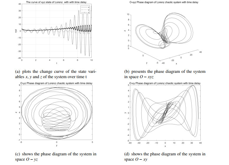
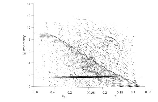
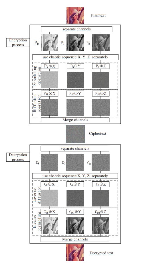
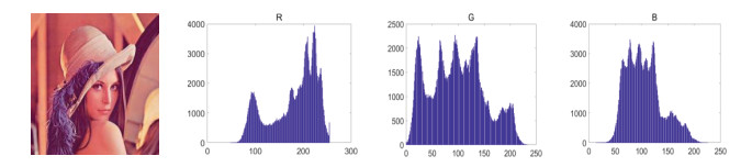
The traditional image encryption technology has the disadvantages of low encryption efficiency and low security. According to the characteristics of image information, an image encryption algorithm based on double time-delay chaos is proposed by combining the delay chaotic system with traditional encryption technology. Because of the infinite dimension and complex dynamic behavior of the delayed chaotic system, it is difficult to be simulated by AI technology. Furthermore time delay and time delay position have also become elements to be considered in the key space. The proposed encryption algorithm has good quality. The stability and the existence condition of Hopf bifurcation of Lorenz system with double delay at the equilibrium point are studied by nonlinear dynamics theory, and the critical delay value of Hopf bifurcation is obtained. The system intercepts the pseudo-random sequence in chaotic state and encrypts the image by means of scrambling operation and diffusion operation. The algorithm is simulated and analyzed from key space size, key sensitivity, plaintext image sensitivity and plaintext histogram. The results show that the algorithm can produce satisfactory scrambling effect and can effectively encrypt and decrypt images without distortion. Moreover, the scheme is not only robust to statistical attacks, selective plaintext attacks and noise, but also has high stability.
- image encryption,
- chaotic encryption,
- double time-delay Lorenz system,
- Hopf bifurcation
Citation: Yuzhen Zhou, Erxi Zhu, Shan Li. An image encryption algorithm based on the double time-delay Lorenz system[J]. Mathematical Biosciences and Engineering, 2023, 20(10): 18491-18522. doi: 10.3934/mbe.2023821

Related Papers:

Abstract

The traditional image encryption technology has the disadvantages of low encryption efficiency and low security. According to the characteristics of image information, an image encryption algorithm based on double time-delay chaos is proposed by combining the delay chaotic system with traditional encryption technology. Because of the infinite dimension and complex dynamic behavior of the delayed chaotic system, it is difficult to be simulated by AI technology. Furthermore time delay and time delay position have also become elements to be considered in the key space. The proposed encryption algorithm has good quality. The stability and the existence condition of Hopf bifurcation of Lorenz system with double delay at the equilibrium point are studied by nonlinear dynamics theory, and the critical delay value of Hopf bifurcation is obtained. The system intercepts the pseudo-random sequence in chaotic state and encrypts the image by means of scrambling operation and diffusion operation. The algorithm is simulated and analyzed from key space size, key sensitivity, plaintext image sensitivity and plaintext histogram. The results show that the algorithm can produce satisfactory scrambling effect and can effectively encrypt and decrypt images without distortion. Moreover, the scheme is not only robust to statistical attacks, selective plaintext attacks and noise, but also has high stability.

References

[1]	M. Bouchaala, C. Ghazel, L. A. Saidane, Enhancing security and efficiency in cloud computing authentication and key agreement scheme based on smart card, J. Supercomput., 78 (2022), 497–522. https://doi.org/10.1007/s11227-021-03857-7 doi: 10.1007/s11227-021-03857-7
[2]	S. Gao, R. Wu, X. Wang, J. Liu, Q. Li, C. Wang, et al., Asynchronous updating Boolean network encryption algorithm, IEEE Trans. Circuits Syst. Video Technol., 33 (2023), 4388–4400. https://doi.org/10.1109/TCSVT.2023.3237136 doi: 10.1109/TCSVT.2023.3237136
[3]	L. Yuan, S. Zheng, Z. Alam, Dynamics analysis and cryptographic application of fractional logistic map, Nonlinear Dyn., 202 (2019), 615–636. https://doi.org/10.1007/s11071-019-04810-3 doi: 10.1007/s11071-019-04810-3
[4]	S. Gao, R. Wu, X. Wang, J. Liu, Q. Li, C. Wang, et al., A 3D model encryption scheme based on a cascaded chaotic system, Signal Process., 202 (2023), 108745. https://doi.org/j.sigpro.2022.108745
[5]	D. Park, S. Hong, N. S. Chang, S. Cho, Efficient implementation of modular multiplication over 192-bit NIST prime for 8-bit AVR-based sensor node, J. Supercomput., 77 (2021), 4852–4870. https://doi.org/10.1007/s11227-020-03441-5 doi: 10.1007/s11227-020-03441-5
[6]	S. Gao, R. Wu, X. Wang, J. Liu, Q. Li, C. Wang, et al., EFR-CSTP: Encryption for face recognition based on the chaos and semi-tensor product theory, Inf. Sci., 621 (2023), 766–781. https://doi.org/10.1016/j.ins.2022.11.121 doi: 10.1016/j.ins.2022.11.121
[7]	R. Wu, S. Gao, X. Wang, J. Liu, Q. Li, C. Wang, et al., AEA-NCS: An audio encryption algorithm based on a nested chaotic system, Chaos Soliton. Fract., 165 (2022), 112770. https://doi.org/10.1016/j.chaos.2022.112770 doi: 10.1016/j.chaos.2022.112770
[8]	W. Diffie, M. E. Hellman, Special feature exhaustive cryptanalysis of the NBS data encryption standard, Computer, 10 (1977), 74–84. https://doi.org/10.1109/C-M.1977.217750 doi: 10.1109/C-M.1977.217750
[9]	M. Monger, The RC6 algorithm is a block cipher that was one of the finalists in the Advanced Encryption Standard (AES) competition sponsored by the National Secu, J. Radiat. Res., 56 (2015), 248–260. https://doi.org/10.1109/IAdCC.2013.6514287 doi: 10.1109/IAdCC.2013.6514287
[10]	M. Robert, On the derivation of a "chaotic" encryption algorithm, Cryptologia, 13 (1989), 29–42. https://doi.org/10.1080/0161-118991863745 doi: 10.1080/0161-118991863745
[11]	H. Asadollahi, M. S. Kamarposhti, E. M. Jandaghi, Image encryption using cellular automata and arnold cat's map, Australian J. Basic Appl. Sci., 5 (2011), 587–593.
[12]	X. Huang, Image encryption algorithm using chaotic Chebyshev generator, Nonlinear Dyn., 67 (2012), 2411–2417. https://doi.org/10.1007/s11071-011-0155-7 doi: 10.1007/s11071-011-0155-7
[13]	X. Wang, L. Liu, Y. Zhang, A novel chaotic block image encryption algorithm based on dynamic random growth technique, Opt. Lasers Eng., 66 (2015), 10–18. https://doi.org/10.1016/j.optlaseng.2014.08.005 doi: 10.1016/j.optlaseng.2014.08.005
[14]	A. Akhshani, A. Akhavan, S. C. Lim, Z. Hassan, An image encryption scheme based on quantum logistic map, Commun. Nonlinear Sci. Numer. Simul., 17 (2012), 4653–4661. https://doi.org/10.1016/j.cnsns.2012.05.033 doi: 10.1016/j.cnsns.2012.05.033
[15]	Y. Guo, J. Yang, B. Liu, Application of chaotic encryption algorithm based on variable parameters in RFID security, EURASIP J. Wirel. Commun. Netw., 2021 (2021), 1–. https://doi.org/10.1186/s13638-021-02023-0 doi: 10.1186/s13638-021-02023-0
[16]	F. Pichler, J. Scharinger, Finite dimensional generalized baker dynamical systems for cryptographic applications, Int. Conf. Comput. Aided Syst. Theor., 1030 (2005), 465–476. https://doi.org/10.1007/BFb0034782 doi: 10.1007/BFb0034782
[17]	G. Ye, K. W. Wong, An efficient chaotic image encryption algorithm based on a generalized Arnold map, Nonlinear Dyn., 69 (2012), 2079–2087. https://doi.org/10.1007/s11071-012-0409-z doi: 10.1007/s11071-012-0409-z
[18]	F. Sun, S. Liu, Z. Li, Q. Zhong, Z. Lü, A novel image encryption scheme based on spatial chaos map, Chaos Soliton. Fract., 38 (2008), 631–640. https://doi.org/10.1016/j.chaos.2008.01.028 doi: 10.1016/j.chaos.2008.01.028
[19]	F. Sun, Z. Lü, S. Liu, A new cryptosystem based on spatial chaotic system, Opt. Commun., 283 (2010), 2066–2073. https://doi.org/10.1016/J.OPTCOM.2010.01.028 doi: 10.1016/J.OPTCOM.2010.01.028
[20]	H. Liu, X. Wang, Color image encryption using spatial bit-level permutation and high-dimension chaotic system, Opt. Commun., 284 (2011), 3895–3903. https://doi.org/10.1016/j.optcom.2011.04.001 doi: 10.1016/j.optcom.2011.04.001
[21]	Z. Zhu, W. Zhang, K. W. Wong, H. Yu, A chaos-based symmetric image encryption scheme using a bit-level permutation, Inf. Sci., 181 (2011), 1171–1186. https://doi.org/10.1016/j.ins.2010.11.009 doi: 10.1016/j.ins.2010.11.009
[22]	P. Manjunath, K. L. Sudha, Chaos image encryption using pixel shuffling, CCSEA, 1 (2011), 169–179. https://doi.org/10.5121/csit.2011.1217 doi: 10.5121/csit.2011.1217
[23]	Y. Jiang, B. Li, A novel image encryption algorithm based on logistic and henon map, 2016 13th International Computer Conference on Wavelet Active Media Technology and Information Processing (ICCWAMTIP), 2016, 66–69. https://doi.org/10.1109/ICCWAMTIP.2016.8079806
[24]	G. Chen, Y. Mao, C. K. Chui, A symmetric image encryption scheme based on 3D chaotic cat maps, Chaos Soliton. Fract., 21 (2004), 749-761. https://doi.org/10.1016/j.chaos.2003.12.022 doi: 10.1016/j.chaos.2003.12.022
[25]	Y. Luo, M. Du, A Novel Digital Image Encryption Scheme Based on Spatial-chaos, J. Convergence Inf. Technol., 7 (2012), 199–207. https://doi.org/10.1016/j.chaos.2008.01.028 doi: 10.1016/j.chaos.2008.01.028
[26]	C. Li, Y. Liu, L. Y. Zhang, M. Chen, Breaking a chaotic image encryption algorithm based on modulo addition and XOR operation, Int. J. Bifurcat. Chaos, 23 (2003), 1350075–1350087. https://doi.org/10.1142/S0218127413500752 doi: 10.1142/S0218127413500752
[27]	C. Gangadhar, K. D. Rao, HYPERCHAOS BASED IMAGE ENCRYPTION, Int. J. Bifurcat. Chaos, 19 (2009), 3833–3839. https://doi.org/10.1142/S021812740902516X doi: 10.1142/S021812740902516X
[28]	Q. Zhang, X. Xue, X. Wei, A novel image encryption algorithm based on DNA subsequence operation, Sci. World J., 2012 (2012), 286741–286751. https://doi.org/10.1100/2012/286741 doi: 10.1100/2012/286741
[29]	S. Lian, J. Sun, Z. Wang, A block cipher based on a suitable use of the chaotic standard map, Chaos Soliton. Fract., 26 (2005), 117–129. https://doi.org/10.1016/j.chaos.2004.11.096 doi: 10.1016/j.chaos.2004.11.096
[30]	H. Mkaouar, O. Boubaker, Chaos synchronization for master slave piecewise linear systems: Application to Chua's circuit, Commun. Nonlinear Sci. Numer. Simul., 17 (2012), 1292–1302. https://doi.org/10.1016/j.cnsns.2011.07.027 doi: 10.1016/j.cnsns.2011.07.027
[31]	L. Chen, H. Yin, T. Huang, L. Yuan, S. Zheng, L. Yin, Chaos in fractional-order discrete neural networks with application to image encryption, Neural Netw., 125 (2020), 174–184. https://doi.org/10.1016/j.neunet.2020.02.008 doi: 10.1016/j.neunet.2020.02.008
[32]	C. Liu, L. Tao, L. Ling, L. Kai, A new chaotic attractor, Chaos Soliton. Fract., 22 (2004), 1031–1038. https://doi.org/10.1016/j.chaos.2004.02.060
[33]	Y. Yu, S. Zhang, Hopf bifurcation in the Lü system, Commun. Nonlinear Sci. Numer. Simul., 17 (2003), 901–906. https://doi.org/10.1016/S0960-0779(02)00573-8 doi: 10.1016/S0960-0779(02)00573-8
[34]	X. Hu, A. Pratap, Z. Zhang, A. Wan, Hopf bifurcation and global exponential stability of an epidemiological smoking model with time delay, Alex. Eng. J., 61 (2022), 2096–2104. https://doi.org/10.1016/j.aej.2021.08.001 doi: 10.1016/j.aej.2021.08.001
[35]	G. Qi, G. Chen, S. Du, Z. Chen, Z. Yuan, Analysis of a new chaotic system, Physica A, 352 (2005), 295–308. https://doi.org/10.1016/J.PHYSA.2004.12.040 doi: 10.1016/J.PHYSA.2004.12.040
[36]	S. N. Chow, J. Mallet-Paret, The Fuller index and global Hopf bifurcation, J. Differ. Equ., 29 (1978), 66–85. https://doi.org/10.1016/0022-0396(78)90041-4 doi: 10.1016/0022-0396(78)90041-4
[37]	X. Huang, Image encryption algorithm using chaotic Chebyshev generator, Nonlinear Dyn., 67 (2012), 2411–2417. https://doi.org/10.1007/s11071-011-0155-7 doi: 10.1007/s11071-011-0155-7
[38]	L. Teng, X. Wang, A bit-level image encryption algorithm based on spatiotemporal chaotic system and self-adaptive, Opt. Commun., 285 (2012), 4048–4054. https://doi.org/10.1016/j.optcom.2012.06.004 doi: 10.1016/j.optcom.2012.06.004
[39]	Z. Parvin, H. Seyedarabi, M. Shamsi, A new secure and sensitive image encryption scheme based on new substitution with chaotic function, Multimed. Tools. Appl., 75 (2014), 10631–10648. https://doi.org/10.1007/s11042-014-2115-y doi: 10.1007/s11042-014-2115-y

Reader Comments

Your name:*

Email:*
© 2023 the Author(s), licensee AIMS Press. This is an open access article distributed under the terms of the Creative Commons Attribution License (http://creativecommons.org/licenses/by/4.0)