Modelling the transmission and control of COVID-19 in Yangzhou city with the implementation of Zero-COVID policy

Juan Li; Wendi Bao; Xianghong Zhang; Yongzhong Song; Zhigui Lin; Huaiping Zhu; Juan Li; Wendi Bao; Xianghong Zhang; Yongzhong Song; Zhigui Lin; Huaiping Zhu

doi:10.3934/mbe.2023703

Mathematical Biosciences and Engineering

2023, Volume 20, Issue 9: 15781-15808. doi: 10.3934/mbe.2023703

Previous Article Next Article

Research article Special Issues

Modelling the transmission and control of COVID-19 in Yangzhou city with the implementation of Zero-COVID policy

1.
School of Computer Science and Technology (School of Artificial Intelligence), Zhejiang Sci-Tech University, Hangzhou 310018, China
2.
College of Science, China University of Petroleum, Qingdao 266580, China
3.
School of Mathematics and Statistics, Southwest University, Chongqing 400715, China
4.
Jiangsu Key Laboratory for NSLSCS, Institute of Mathematics School of Mathematics Science Nanjing Normal University, Nanjing 210023, China
5.
School of Mathematical Science, Yangzhou University, Yangzhou 225002, China
6.
LAMPS and Center for Diseases Modeling (CDM), Department of Mathematics and Statistics, York University, Toronto M3J 1P3, ON, Canada

Academic Editor: Xiang-Sheng Wang

Received: 02 June 2023 Revised: 18 June 2023 Accepted: 25 June 2023 Published: 31 July 2023

In the fight against the COVID-19 pandemic, China has long adhered to the "Dynamic Zero COVID-19" strategy till the end of 2022. To understand the mechanism of this strategy, we used the case of the Yangzhou summer outbreak in 2021 and a multi-stage dynamical model incorporating city-wide and key area testing-trace-isolation (TTI) strategies. We defined two time-varying indexes for measuring the disease transmission risk and the public health prevention and control force, respectively, which allowed us to explore the mechanisms of TTI policies. Integrating with the historical data and literature parameter values, we first estimated the parameters and then quantified the relevant indexes over time. The findings showed that multiple rounds of rapid testing were one of the critical measures to overcome the outbreak in Yangzhou within one month. In addition, we compared the impact of the duration of the free transmission stage, tracking rate, testing interval and precise division of key areas on the epidemiological indicators, including the final sizes of infections and isolations, peak value, peak arrival time and epidemic duration and the minimum round of testing. Our results suggest that the early detection of the epidemic, an improved efficiency of tracking, and a reduced duration of each test play a positive role in restraining COVID-19; however, a considerable investment of resources was essential to achieve a significant effect quickly.
Citation: Juan Li, Wendi Bao, Xianghong Zhang, Yongzhong Song, Zhigui Lin, Huaiping Zhu. Modelling the transmission and control of COVID-19 in Yangzhou city with the implementation of Zero-COVID policy[J]. Mathematical Biosciences and Engineering, 2023, 20(9): 15781-15808. doi: 10.3934/mbe.2023703

Related Papers:

Abstract

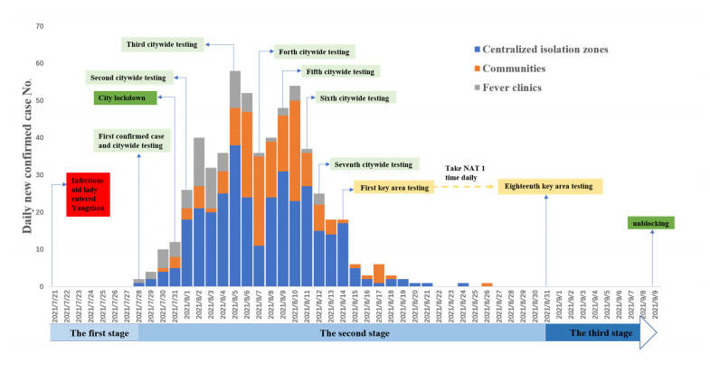
In the fight against the COVID-19 pandemic, China has long adhered to the "Dynamic Zero COVID-19" strategy till the end of 2022. To understand the mechanism of this strategy, we used the case of the Yangzhou summer outbreak in 2021 and a multi-stage dynamical model incorporating city-wide and key area testing-trace-isolation (TTI) strategies. We defined two time-varying indexes for measuring the disease transmission risk and the public health prevention and control force, respectively, which allowed us to explore the mechanisms of TTI policies. Integrating with the historical data and literature parameter values, we first estimated the parameters and then quantified the relevant indexes over time. The findings showed that multiple rounds of rapid testing were one of the critical measures to overcome the outbreak in Yangzhou within one month. In addition, we compared the impact of the duration of the free transmission stage, tracking rate, testing interval and precise division of key areas on the epidemiological indicators, including the final sizes of infections and isolations, peak value, peak arrival time and epidemic duration and the minimum round of testing. Our results suggest that the early detection of the epidemic, an improved efficiency of tracking, and a reduced duration of each test play a positive role in restraining COVID-19; however, a considerable investment of resources was essential to achieve a significant effect quickly.

References

[1]	CSSE: COVID-19 Dashboard, Johns Hopkins University (JHU), 2022. Available from: https://www.arcgis.com/apps/dashboards/bda7594740fd40299423467b48e9ecf6.
[2]	WHO: Tracking SARS-CoV-2 variants, 2022. Available from: https://www.who.int/en/activities/tracking-SARS-CoV-2-variants/.
[3]	T. K. Burki, Omicron variant and booster COVID-19 vaccines, Lancet Respir. Med., 10 (2022). https://doi.org/10.1016/S2213-2600(21)00559-2 doi: 10.1016/S2213-2600(21)00559-2
[4]	Y. Liu, J. Rocklöv, The reproductive number of the Delta variant of SARS-CoV-2 is far higher compared to the ancestral SARS-CoV-2 virus, J. Travel Med., 28 (2021), 1–3. https://doi.org/10.1093/jtm/taab124 doi: 10.1093/jtm/taab124
[5]	MMWR: Centers for Disease Control and Prevention, 2022. Available from: https://www.cdc.gov/mmwr/volumes/71/wr/mm7104e4.htm.
[6]	O. Barnes, J. Burn-Murdoch, Omicron's less severe cases prompt cautious optimism in South Africa, 2021. Available from: https://www.ft.com/content/d315be08-cda0-462b-85ec-811290ad488e.
[7]	WHO: WHO Director-General's opening remarks at the media briefing – 5 May 2023, 2023. Available from: https://www.who.int/director-general/speeches/detail/who-director-general-s-opening-remarks-at-the-media-briefing---5-may-2023.
[8]	M. Oliu-Barton, B. S. R. Pradelski, Y. Algan, M. G. Baker, A. Binagwaho, G. J. Dore, et al., Elimination versus mitigation of SARS-CoV-2 in the presence of effective vaccines, Lancet Global Health, 10 (2022), e142–e147, 2022. https://doi.org/10.1016/S2214-109X(21)00494-0 doi: 10.1016/S2214-109X(21)00494-0
[9]	M. Oliu-Barton, B. S. R. Pradelski, P. Aghion, P. Artus, I. Kickbusch, J. V. Lazarus, et al., SARS-CoV-2 elimination, not mitigation, creates best outcomes for health, the economy, and civil liberties, Lancet, 397 (2021), 12–18. https://doi.org/10.1016/S0140-6736(21)00978-8 doi: 10.1016/S0140-6736(21)00978-8
[10]	W. Liang, M. Liu, J. Liu, Y. Wang, J. Wu, X. Liu, The dynamic COVID-zero strategy on prevention and control of COVID-19 in China (in Chinese), Chin. Med. J., 102 (2022), 239–242. https://doi.org/10.3760/cma.j.cn112137-20211205-02710 doi: 10.3760/cma.j.cn112137-20211205-02710
[11]	Coexist with COVID-19' for only ten days, the number of critically ill cases in Korea has reached a new high (in Chinese), 2021. Available from: https://baijiahao.baidu.com/s?id = 1716037339938236108 & wfr = spider & for = pc.
[12]	Y. Xing, G. Wong, W. Ni, X. Hu, Q. Xing, Rapid response to an outbreak in Qingdao, China, N. Engl. J. Med., 383 (2020), e129. https://doi.org/10.1056/nejmc2032361 doi: 10.1056/nejmc2032361
[13]	Z. Wu, Q. Wang, J. Zhao, P. Yang, J. M. McGoogan, Z. Feng, et al., Time course of a second outbreak of COVID-19 in Beijing, China, June-July 2020, JAMA, 324 (2020), 1458−1459. https://doi.org/10.1001/jama.2020.15894 doi: 10.1001/jama.2020.15894
[14]	Z. Li, F. Liu, J. Cui, Z. Peng, Z. Chang, S. Lai, et al., Comprehensive large-scale nucleic acid–testing strategies support China's sustained containment of COVID-19, Nat. Med., 27 (2021), 740–742. https://doi.org/10.1038/s41591-021-01308-7 doi: 10.1038/s41591-021-01308-7
[15]	New Coronavirus Pneumonia Diagnosis and Treatment Plan (Trial Version 8) (in Chinese), National Health Commission of the People's Republic of China, 2020. Available from: http://www.nhc.gov.cn/yzygj/s7653p/202008/0a7bdf12bd4b46e5bd28ca7f9a7f5e5a.shtml.
[16]	Y. Zhang, C. You, X. Gai, X. Zhou, On coexistence with COVID-19: estimations and perspectives, China CDC Wkly, 3 (2021), 1057–1061. https://doi.org/10.46234/ccdcw2021.245 doi: 10.46234/ccdcw2021.245
[17]	B. Tang, F. Xia, S. Tang, N. L. Bragazzi, Q. Li, X. Sun, et al., The effectiveness of quarantine and isolation determine the trend of the COVID-19 epidemic in the final phase of the current outbreak in China, Int. J. Infect. Dis., 95 (2020), 288–293. https://doi.org/10.1016/j.ijid.2020.03.018 doi: 10.1016/j.ijid.2020.03.018
[18]	C. Hou, J. Chen, Y. Zhou, L. Hua, J. Yuan, S. He, et al., The effectiveness of quarantine of Wuhan city against the Corona Virus Disease 2019 (COVID-19): a well-mixed SEIR model analysis, J. Med. Virol., 92 (2020), 841–848. https://doi.org/10.1002/jmv.25827 doi: 10.1002/jmv.25827
[19]	K. Shimizu, T. Kuniya, Y. Tokuda, Modeling population-wide testing of SARS-CoV-2 for containing COVID-19 pandemic in Okinawa, Japan, J. Gen. Fam. Med., 22 (2021), 173–181. https://doi.org/10.1002/jgf2.439 doi: 10.1002/jgf2.439
[20]	A. Aleta, D. Martín-Corral, A. P. Y. Piontti, M. Ajelli, M. Litvinova, M. Chinazzi, et al., Modelling the impact of testing, contact tracing and household quarantine on second waves of COVID-19, Nat. Hum. Behav., 4 (2020), 964–971. https://doi.org/10.1038/s41562-020-0931-9 doi: 10.1038/s41562-020-0931-9
[21]	T. Colbourn, W. Waites, J. Panovska-Griffiths, D. Manheim, S. Sturniolo, G. Colbourn, et al., Modelling the health and economic impacts of population-wide testing, contact tracing and isolation (PTTI) strategies for COVID-19 in the UK, SSRN Electron. J., 9 (2020). https://doi.org/10.2139/ssrn.3627273 doi: 10.2139/ssrn.3627273
[22]	A. J. Kucharski, P. Klepac, A. J. K. Conlan, S. M. Kissler, M. L. Tang, H. Fry, et al., Effectiveness of isolation, testing, contact tracing, and physical distancing on reducing transmission of SARS-CoV-2 in different settings: a mathematical modelling study, Lancet Infect. Dis., 20 (2020), 1151–1160. https://doi.org/10.1016/s1473-3099(20)30457-6 doi: 10.1016/s1473-3099(20)30457-6
[23]	S. Contreras, J. Dehning, M. Loidolt, J. Zierenberg, F. P. Spitzner, J. H. Urrea-Quintero, et al., The challenges of containing SARS-CoV-2 via test-trace-and-isolate, Nat. Commun., 12 (2021), 378. https://doi.org/10.1038/s41467-020-20699-8 doi: 10.1038/s41467-020-20699-8
[24]	Yangzhou city health and family planning commission website, 2021. Available from: http://wjw.yangzhou.gov.cn/.
[25]	The paper news official website, 2021. Available from: ttps: //www.thepaper.cn/.
[26]	A. Holborow, H. Asad, L. Porter, P. Tidswell, C. Johnston, I. Blyth, et al., The clinical sensitivity of a single SARS-CoV-2 upper respiratory tract RT-PCR test for diagnosing COVID-19 using convalescent antibody as a comparator, Clin. Med., 20 (2020), 6. https://doi.org/10.7861/clinmed.2020-0555 doi: 10.7861/clinmed.2020-0555
[27]	J. Chhatwal, Y. Xiao, P. Mueller, M. Adee, O. O. Dalgic, M. A. Ladd, et al., Changing dynamics of COVID-19 in the U.S. with the emergence of the Delta variant: projections of the COVID-19 simulator, medRxiv, 2021. https://doi.org/10.1101/2021.08.11.21261845 doi: 10.1101/2021.08.11.21261845
[28]	B. Li, A. Deng, K. Li, Y. Hu, Z. Li, Y. Shi, et al., Viral infection and transmission in a large well-traced outbreak caused by the Delta SARS-CoV-2 variant, Nat. Commun., 13 (2022). https://doi.org/10.1038/s41467-022-28089-y doi: 10.1038/s41467-022-28089-y
[29]	M. Du, M. Liu, J. Liu, Progress in research of epidemiologic feature and control of SARS-CoV-2 Delta variant (in Chinese), Chin. J. Epidemiol., 42 (2021), 1774–1779. https://doi.org/10.3760/cma.j.cn112338-20210808-00619 doi: 10.3760/cma.j.cn112338-20210808-00619
[30]	P. Dreessche, J. Watmough, Reproduction numbers and sub-threshold endemic equilibria for compartmental models of disease transmission, Math. Biosci., 180 (2022), 29–48. https://doi.org/10.1016/S0025-5564(02)00108-6 doi: 10.1016/S0025-5564(02)00108-6
[31]	H. R. Thieme, Spectral bound and reproduction number for infinite dimensional population structure and time heterogeneity, SIAM J. Appl. Math., 70 (2009), 188–211. https://doi.org/10.1137/080732870 doi: 10.1137/080732870
[32]	A. Cintrón-Arias, C. Castillo-Chávez, L. M. A. Bettencourt, A. L. Lloyd, H. T. Banks, The estimation of the effective reproductive number from disease outbreak data, Math. Biosci. Eng., 6 (2009), 261–282. https://doi.org/10.3934/mbe.2009.6.261 doi: 10.3934/mbe.2009.6.261
[33]	H. Haario, M. Laine, A. Mira, E. Saksman, DRAM: efficient adaptive MCMC, Stat. Comput., 16 (2006), 339–354. https://doi.org/10.1007/s11222-006-9438-0 doi: 10.1007/s11222-006-9438-0
[34]	M. D. Mckay, R. J. Beckman, W. J. Conover, A comparison of three methods for selecting values of input variables in the analysis of output from a computer code, Technometrics, 21 (1979), 239–245. https://doi.org/10.1080/00401706.2000.10485979 doi: 10.1080/00401706.2000.10485979
[35]	Guidelines for Organization of Regional Novel Coronavirus Nucleic Acid Tests (Third Edition) (in Chinese), 2022. Available from: http://www.nhc.gov.cn/yzygj/s7659/202203/b5aaa96dfe1b4f14b19bf2f888a10673.shtml.
[36]	J. Qi, D. Zhang, X. Zhang, T. Takana, Y. Pan, P. Yin, et al., Short- and medium-term impacts of strict anti-contagion policies on non-COVID-19 mortality in China, Nat. Hum. Behav., 6 (2022), 55–63. https://doi.org/10.1038/s41562-021-01189-3 doi: 10.1038/s41562-021-01189-3

Reader Comments

Your name:*

Email:*
© 2023 the Author(s), licensee AIMS Press. This is an open access article distributed under the terms of the Creative Commons Attribution License (http://creativecommons.org/licenses/by/4.0)