There are approximately 2.2 billion people around the world with varying degrees of visual impairments. Among them, individuals with severe visual impairments predominantly rely on hearing and touch to gather external information. At present, there are limited reading materials for the visually impaired, mostly in the form of audio or text, which cannot satisfy the needs for the visually impaired to comprehend graphical content. Although many scholars have devoted their efforts to investigating methods for converting visual images into tactile graphics, tactile graphic translation fails to meet the reading needs of visually impaired individuals due to image type diversity and limitations in image recognition technology. The primary goal of this paper is to enable the visually impaired to gain a greater understanding of the natural sciences by transforming images of mathematical functions into an electronic format for the production of tactile graphics. In an effort to enhance the accuracy and efficiency of graph element recognition and segmentation of function graphs, this paper proposes an MA Mask R-CNN model which utilizes MA ConvNeXt as its improved feature extraction backbone network and MA BiFPN as its improved feature fusion network. The MA ConvNeXt is a novel feature extraction network proposed in this paper, while the MA BiFPN is a novel feature fusion network introduced in this paper. This model combines the information of local relations, global relations and different channels to form an attention mechanism that is able to establish multiple connections, thus increasing the detection capability of the original Mask R-CNN model on slender and multi-type targets by combining a variety of multi-scale features. Finally, the experimental results show that MA Mask R-CNN attains an 89.6% mAP value for target detection and 72.3% mAP value for target segmentation in the instance segmentation of function graphs. This results in a 9% mAP improvement for target detection and 12.8% mAP improvement for target segmentation compared to the original Mask R-CNN.
Citation: Jiale Lu, Jianjun Chen, Taihua Xu, Jingjing Song, Xibei Yang. Element detection and segmentation of mathematical function graphs based on improved Mask R-CNN[J]. Mathematical Biosciences and Engineering, 2023, 20(7): 12772-12801. doi: 10.3934/mbe.2023570
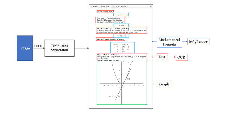
There are approximately 2.2 billion people around the world with varying degrees of visual impairments. Among them, individuals with severe visual impairments predominantly rely on hearing and touch to gather external information. At present, there are limited reading materials for the visually impaired, mostly in the form of audio or text, which cannot satisfy the needs for the visually impaired to comprehend graphical content. Although many scholars have devoted their efforts to investigating methods for converting visual images into tactile graphics, tactile graphic translation fails to meet the reading needs of visually impaired individuals due to image type diversity and limitations in image recognition technology. The primary goal of this paper is to enable the visually impaired to gain a greater understanding of the natural sciences by transforming images of mathematical functions into an electronic format for the production of tactile graphics. In an effort to enhance the accuracy and efficiency of graph element recognition and segmentation of function graphs, this paper proposes an MA Mask R-CNN model which utilizes MA ConvNeXt as its improved feature extraction backbone network and MA BiFPN as its improved feature fusion network. The MA ConvNeXt is a novel feature extraction network proposed in this paper, while the MA BiFPN is a novel feature fusion network introduced in this paper. This model combines the information of local relations, global relations and different channels to form an attention mechanism that is able to establish multiple connections, thus increasing the detection capability of the original Mask R-CNN model on slender and multi-type targets by combining a variety of multi-scale features. Finally, the experimental results show that MA Mask R-CNN attains an 89.6% mAP value for target detection and 72.3% mAP value for target segmentation in the instance segmentation of function graphs. This results in a 9% mAP improvement for target detection and 12.8% mAP improvement for target segmentation compared to the original Mask R-CNN.

| [1] | World Health Organization, World Report on Vision, 2019. Available from: https://www.who.int/publications/i/item/world-report-on-vision. |
| [2] | K. Han, Y. Liu, F. Yuan, The tactile graphics representation and its design application for the visually impaired, Design, 4 (2015), 18–19. |
| [3] | D. Wu, J. Gan, Assistant haptic interaction technology for blind Internet user, J. Eng. Design, 17 (2010), 128–133. |
| [4] | X. Li, Reading resources for the blind and the present situation of reading promotion in China, New Century Lib., 5 (2013), 19–22. |
| [5] |
S. Spooner, "What page, Miss?" enhancing text accessibility with DAISY (Digital Accessible Information System), J. Visual Impairment Blindness, 108 (2014), 201–211. https://doi.org/10.1177/0145482X1410800304 doi: 10.1177/0145482X1410800304

|
| [6] |
S. Suksakulchai, S. Chaisanit, A daisy book production system over the internet, J. Commun. Comput., 8 (2011), 744–750. https://doi.org/10.1038/sj.bdj.4800904 doi: 10.1038/sj.bdj.4800904
|
| [7] | R. Zhang, Digital accessible information system and its development trend, Discovering Value, 6 (2010), 304. |
| [8] |
A. Quint, Scalable vector graphics, IEEE Multimedia, 10 (2003), 99–102. https://doi.org/10.1109/MMUL.2003.1218261 doi: 10.1109/MMUL.2003.1218261
|
| [9] | G. Browne, Ebook indexes, EPUB and the international digital publishing forum, Online Curr., 26 (2012), 127–130. |
| [10] | P. P. Rege, A. C. Chandrakar, Text-image separation in document images using boundary/perimeter detection, ACEEE Int. J. Signal Image Process., 3 (2012), 10–14. https://doi.org/01.IJSIP.03.01.70 |
| [11] | P. Lyu, M. Liao, C. Yao, W. Wu, X. Bai, Mask textspotter: An end-to-end trainable neural network for spotting text with arbitrary shapes, in Proceedings of the European Conference on Computer Vision (ECCV), (2018), 67–83. https://doi.org/10.48550/arXiv.1807.02242 |
| [12] | Y. Baek, B. Lee, D. Han, S. Yun, H. Lee, Character region awareness for text detection, in Proceedings of the IEEE/CVF Conference on Computer Vision and Pattern Recognition, (2019), 9365–9374. https://doi.org/10.1109/CVPR.2019.00959 |
| [13] |
J. Memon, M. Sami, R. A. Khan, M. Uddin, Handwritten optical character recognition (OCR): A comprehensive systematic literature review (SLR), IEEE Access, 8 (2020), 142642–142668. https://doi.org/10.1109/ACCESS.2020.3012542 doi: 10.1109/ACCESS.2020.3012542
|
| [14] |
T. Hegghammer, OCR with Tesseract, Amazon Textract, and Google Document AI: a benchmarking experiment, J. Comput. Social Sci., 5 (2022), 861–882. https://doi.org/10.1007/s42001-021-00149-1 doi: 10.1007/s42001-021-00149-1
|
| [15] | X. Zhou, C. Yao, H. Wen, Y. Wang, S. Zhou, W. He, et al., East: an efficient and accurate scene text detector, in Proceedings of the IEEE Conference on Computer Vision and Pattern Recognition, (2017), 5551–5560. https://doi.org/10.1109/CVPR.2017.283 |
| [16] | M. Suzuki, T. Kanahori, N. Ohtake, K. Yamaguchi, An integrated OCR software for mathematical documents and its output with accessibility, in International Conference on Computers for Handicapped Persons, (2004), 648–655. https://doi.org/10.1007/978-3-540-27817-7_97 |
| [17] | M. Suzuki, Pen-Based Mathematical Computing Organizers, Stephen Watt and Clare So, (2005), 60. |
| [18] |
Z. Wang, J. C. Liu, Translating math formula images to LaTeX sequences using deep neural networks with sequence-level training, Int. J. Doc. Anal. Recogn., 24 (2021), 63–75. https://doi.org/10.1007/s10032-020-00360-2 doi: 10.1007/s10032-020-00360-2
|
| [19] | O. Vinyals, A. Toshev, S. Bengio, D. Erhan, Show and tell: A neural image caption generator, in Proceedings of the IEEE Conference on Computer Vision and Pattern Recognition, (2015), 3156–3164. https://doi.org/10.1109/CVPR.2015.7298935 |
| [20] | Y. Wang, J. Xu, Y. Sun, End-to-end transformer based model for image captioning, in Proceedings of the AAAI Conference on Artificial Intelligence, 36 (2022), 2585–2594. https://doi.org/10.1609/aaai.v36i3.20160 |
| [21] |
T. Fuda, S. Omachi, H. Aso, Recognition of line graph images in documents by tracing connected components, Syst. Comput. Jpn., 38 (2007), 103–114. https://doi.org/10.1002/scj.10615 doi: 10.1002/scj.10615
|
| [22] |
S. Shimada, S. Kakumoto, M. Ejiri, A recognition algorithm of dashed and chained lines for automatic inputting of drawings, IEICE Trans. Inf. Syst., 18 (1986), 759–770. https://doi.org/10.1002/scj.4690180603 doi: 10.1002/scj.4690180603
|
| [23] | N. Yokokura, T. Watanabe, Recognition of business bar-graphs using layout structure knowledge, J. Inf. Process., 40 (1999), 2954–2966. |
| [24] | M. Yo, T. Kawahara, R. Fukuda, Handwriting graphics input system for high school mathematics, IEICE Tech. Rep., 291 (2004), 43–48. |
| [25] | A. Balaji, T. Ramanathan, V. Sonathi, Chart-text: A fully automated chart image descriptor, preprint, arXiv: 1812.10636. https://doi.org/10.48550/arXiv.1812.10636 |
| [26] |
J. Chen, N. Takagi, Development of a method for extracting and recognizing graph elements in mathematical graphs for automating translation of tactile graphics, J. Jpn. Soc. Fuzzy Theory Intell. Inf., 26 (2014), 593–605. https://doi.org/10.3156/jsoft.26.593 doi: 10.3156/jsoft.26.593
|
| [27] |
J. Staker, K. Marshall, R. Abel, C. M. McQuaw, Molecular structure extraction from documents using deep learning, J. Chem. Inf. Model., 59 (2019), 1017–1029. https://doi.org/10.1021/acs.jcim.8b00669 doi: 10.1021/acs.jcim.8b00669
|
| [28] |
M. Oldenhof, A. Arany, Y. Moreau, J. Simm, ChemGrapher: optical graph recognition of chemical compounds by deep learning, J. Chem. Inf. Model., 60 (2020), 4506–4517. https://doi.org/10.1021/acs.jcim.0c00459 doi: 10.1021/acs.jcim.0c00459
|
| [29] | A. Vaswani, N. Shazeer, N. Parmar, J. Uszkoreit, L. Jones, A. N. Gomez, et al., Attention is all you need, in Advances in Neural Information Processing Systems, 30 (2017), 5998–6008. https://doi.org/10.48550/arXiv.1706.03762 |
| [30] | A. Dosovitskiy, L. Beyer, A. Kolesnikov, D. Weissenborn, X. Zhai, T. Unterthiner, et al., An image is worth 16x16 words: Transformers for image recognition at scale, preprint, arXiv: 2010.11929. https://doi.org/10.48550/arXiv.2010.11929 |
| [31] | Z. Liu, Y. Lin, Y. Cao, H. Hu, Y. Wei, Z. Zhang, et al., Swin transformer: Hierarchical vision transformer using shifted windows, in Proceedings of the IEEE/CVF International Conference on Computer Vision, (2021), 10012–10022. https://doi.org/10.1109/ICCV48922.2021.00986 |
| [32] | Z. Liu, H. Mao, C. Wu, C. Feichtenhofer, T. Darrell, S. Xie, A convnet for the 2020s, in Proceedings of the IEEE/CVF Conference on Computer Vision and Pattern Recognition, (2022), 11976–11986. https://doi.org/10.1109/CVPR52688.2022.01167 |
| [33] | M. Tan, R. Pang, Q. V. Le, Efficientdet: Scalable and efficient object detection, in Proceedings of the IEEE/CVF Conference on Computer Vision and Pattern Recognition, (2020), 10781–10790. https://doi.org/10.1109/CVPR42600.2020.01079 |
| [34] | K. He, G. Gkioxari, P. Dollár, R. Girshick, Mask R-CNN, in Proceedings of the IEEE International Conference on Computer Vision, 42 (2017), 2961–2969. https://doi.org/10.1109/TPAMI.2018.2844175 |
| [35] | L. Chen, Y. Zhu, G. Papandreou, F. Schroff, H. Adam, Encoder-decoder with atrous separable convolution for semantic image segmentation, in Proceedings of the European Conference on Computer Vision (ECCV), 40 (2018), 801–818. https://doi.org/10.1109/TPAMI.2017.2699184 |
| [36] | J. Liu, W. Zhang, Y. Tang, J. Tang, G. Wu, Residual feature aggregation network for image super-resolution, in Proceedings of the IEEE/CVF Conference on Computer Vision and Pattern Recognition, (2020), 2359–2368. https://doi.org/10.1109/CVPR42600.2020.00243 |
| [37] | S. Ren, K. He, R. Girshick, J. Sun, Faster R-CNN: Towards real-time object detection with region proposal networks, in Advances in Neural Information Processing Systems, (2015), 28. https://doi.org/10.48550/arXiv.1506.01497 |
| [38] | K. He, X. Zhang, S. Ren, J. Sun, Deep residual learning for image recognition, in Proceedings of the IEEE Conference on Computer Vision and Pattern Recognition, (2016), 770–778. https://doi.org/10.1109/CVPR.2016.90 |
| [39] | T. Lin, P. Dollár, R. Girshick, K. He, B. Hariharan, S. Belongie, Feature pyramid networks for object detection, in Proceedings of the IEEE/CVF Conference on Computer Vision and Pattern Recognition, (2017), 936–944. https://doi.org/10.1109/CVPR.2017.106 |
| [40] | A. Kirillov, Y. Wu, K. He, R. Girshick, PointRend: Image segmentation as rendering, in Proceedings of the IEEE/CVF Conference on Computer Vision and Pattern Recognition, (2020), 9799–9808. https://doi.org/10.1109/CVPR42600.2020.00982 |
| [41] | C. Szegedy, V. Vanhoucke, S. Ioffe, J. Shlens, Z. Wojna, Rethinking the inception architecture for computer vision, in Proceedings of the IEEE Conference on Computer Vision and Pattern Recognition, (2016), 2818–2826. https://doi.org/10.1109/CVPR.2016.308 |
| [42] | Cambridge International Examinations, IGCSE Guide Additional Mathematics Examples & Practice Book 1, Curriculum Planning and Development, 2021. |
| [43] |
D. Bolya, C. Zhou, F. Xiao, Y. J. Lee, Yolact++: Better real-time instance segmentation, IEEE Trans. Pattern Anal. Mach. Intell., 44 (2020). https://doi.org/10.1109/TPAMI.2020.3014297 doi: 10.1109/TPAMI.2020.3014297
|
| [44] | S. Liu, L. Qi, H. Qin, J. Shi, J. Jia, Path aggregation network for instance segmentation, in Proceedings of the IEEE Conference on Computer Vision and Pattern Recognition, (2018), 8759–8768. https://doi.org/10.1109/CVPR.2018.00913 |
| [45] | H. Chen, K. Sun, Z. Tian, C. Shen, Y. Huang, Y. Yan, Blendmask: Top-down meets bottom-up for instance segmentation, in Proceedings of the IEEE/CVF Conference on Computer Vision and Pattern Recognition, (2020), 8573–8581. https://doi.org/10.1109/CVPR42600.2020.00860 |
| [46] | F. Li, H. Zhang, H. Xu, S. Liu, L. Zhang, L. M. Ni, et al., Mask dino: Towards a unified transformer-based framework for object detection and segmentation, in Proceedings of the IEEE Conference on Computer Vision and Pattern Recognition, (2022), 3041–3050. https://doi.org/10.48550/arXiv.2206.02777 |
| [47] | R. R. Selvaraju, M. Cogswell, A. Das, R. V edantam, D. Parikh, D. Batra, Grad-cam: Visual explanations from deep networks via gradient-based localization, in Proceedings of the IEEE International Conference on Computer Vision, (2017), 618–626. https://doi.org/10.1007/s11263-019-01228-7 |
| [48] | X. Zhu, H. Hu, S. Lin, J. Dai, Deformable convnets v2: More deformable, better results, in Proceedings of the IEEE/CVF Conference on Computer Vision and Pattern Recognition, (2019), 9308–9316. https://doi.org/10.1109/CVPR.2019.00953 |


Figures(15) / Tables(5)

Jiale Lu, Jianjun Chen, Taihua Xu, Jingjing Song, Xibei Yang. Element detection and segmentation of mathematical function graphs based on improved Mask R-CNN[J]. Mathematical Biosciences and Engineering, 2023, 20(7): 12772-12801. doi: 10.3934/mbe.2023570


 DownLoad: