Non-small cell lung cancer (NSCLC) is heterogeneous. Molecular subtyping based on the gene expression profiles is an effective technique for diagnosing and determining the prognosis of NSCLC patients.
Here, we downloaded the NSCLC expression profiles from The Cancer Genome Atlas and the Gene Expression Omnibus databases. ConsensusClusterPlus was used to derive the molecular subtypes based on long-chain noncoding RNA (lncRNA) associated with the PD-1-related pathway. The LIMMA package and least absolute shrinkage and selection operator (LASSO)-Cox analysis were used to construct the prognostic risk model. The nomogram was constructed to predict the clinical outcomes, followed by decision curve analysis (DCA) to validate the reliability of this nomogram.
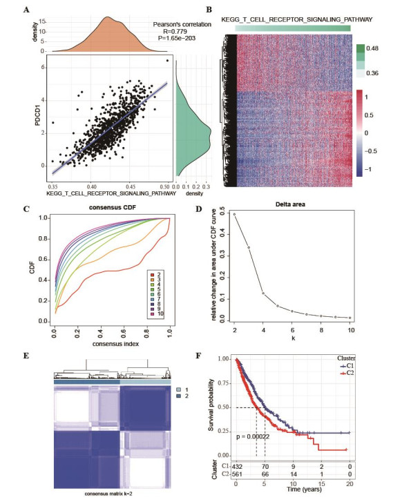
We discovered that PD-1 was strongly and positively linked to the T-cell receptor signaling pathway. Furthermore, we identified two NSCLC molecular subtypes yielding a significantly distinctive prognosis. Subsequently, we developed and validated the 13-lncRNA-based prognostic risk model in the four datasets with high AUC values. Patients with low-risk showed a better survival rate and were more sensitive to PD-1 treatment. Nomogram construction combined with DCA revealed that the risk score model could accurately predict the prognosis of NSCLC patients.
This study demonstrated that lncRNAs engaged in the T-cell receptor signaling pathway played a significant role in the onset and development of NSCLC, and that they could influence the sensitivity to PD-1 treatment. In addition, the 13 lncRNA model was effective in assisting clinical treatment decision-making and prognosis evaluation.
Citation: Hejian Chen, Shuiyu Xu, Yuhong Zhang, Peifeng Chen. Systematic analysis of lncRNA gene characteristics based on PD-1 immune related pathway for the prediction of non-small cell lung cancer prognosis[J]. Mathematical Biosciences and Engineering, 2023, 20(6): 9818-9838. doi: 10.3934/mbe.2023430
Non-small cell lung cancer (NSCLC) is heterogeneous. Molecular subtyping based on the gene expression profiles is an effective technique for diagnosing and determining the prognosis of NSCLC patients.
Here, we downloaded the NSCLC expression profiles from The Cancer Genome Atlas and the Gene Expression Omnibus databases. ConsensusClusterPlus was used to derive the molecular subtypes based on long-chain noncoding RNA (lncRNA) associated with the PD-1-related pathway. The LIMMA package and least absolute shrinkage and selection operator (LASSO)-Cox analysis were used to construct the prognostic risk model. The nomogram was constructed to predict the clinical outcomes, followed by decision curve analysis (DCA) to validate the reliability of this nomogram.
We discovered that PD-1 was strongly and positively linked to the T-cell receptor signaling pathway. Furthermore, we identified two NSCLC molecular subtypes yielding a significantly distinctive prognosis. Subsequently, we developed and validated the 13-lncRNA-based prognostic risk model in the four datasets with high AUC values. Patients with low-risk showed a better survival rate and were more sensitive to PD-1 treatment. Nomogram construction combined with DCA revealed that the risk score model could accurately predict the prognosis of NSCLC patients.
This study demonstrated that lncRNAs engaged in the T-cell receptor signaling pathway played a significant role in the onset and development of NSCLC, and that they could influence the sensitivity to PD-1 treatment. In addition, the 13 lncRNA model was effective in assisting clinical treatment decision-making and prognosis evaluation.

| [1] |
R. L. Siegel, K. D. Miller, H. E. Fuchs, A. Jemal, Cancer Statistics, 2021, CA Cancer J. Clin., 71 (2021), 7–33. https://doi.org/10.3322/caac.21654 doi: 10.3322/caac.21654

|
| [2] |
F. Islami, A. G. Sauer, K. D. Miller, R. L. Siegel, S. A. Fedewa, E. J. Jacobs, et al., Proportion and number of cancer cases and deaths attributable to potentially modifiable risk factors in the United States, CA Cancer J. Clin., 68 (2018), 31–54. https://doi.org/10.3322/caac.21440 doi: 10.3322/caac.21440
|
| [3] |
M. Zheng, Classification and pathology of lung cancer, Surg. Oncol. Clin., 25 (2016), 447–468. https://doi.org/10.1016/j.soc.2016.02.003 doi: 10.1016/j.soc.2016.02.003
|
| [4] |
M. Wang, R. S. Herbst, C. Boshoff, Toward personalized treatment approaches for non-small-cell lung cancer, Nat. Med., 27 (2021), 1345–1356. https://doi.org/10.1038/s41591-021-01450-2 doi: 10.1038/s41591-021-01450-2
|
| [5] |
M. MacManus, F. Hegi-Johnson, Overcoming immunotherapy resistance in NSCLC, Lancet Oncol., 23 (2022), 191–193. https://doi.org/10.1016/S1470-2045(21)00711-7 doi: 10.1016/S1470-2045(21)00711-7
|
| [6] |
A. Insa, P. Martín-Martorell, R. D. Liello, M. Fasano, G. Martini, S. Napolitano, et al., Which treatment after first line therapy in NSCLC patients without genetic alterations in the era of immunotherapy? Crit. Rev. Oncol. Hematol., 169 (2022), 103538. https://doi.org/10.1016/j.critrevonc.2021.103538 doi: 10.1016/j.critrevonc.2021.103538
|
| [7] |
F. Xie, M. Xu, J. Lu, L. Mao, S. Wang, The role of exosomal PD-L1 in tumor progression and immunotherapy, Mol. Cancer, 18 (2019), 146. https://doi.org/10.1186/s12943-019-1074-3 doi: 10.1186/s12943-019-1074-3
|
| [8] |
M. Niu, M. Yi, N. Li, S. Luo, K. Wu, Predictive biomarkers of anti-PD-1/PD-L1 therapy in NSCLC, Exp. Hematol. Oncol., 10 (2021), 18. https://doi.org/10.1186/s40164-021-00211-8 doi: 10.1186/s40164-021-00211-8
|
| [9] |
P. Yu, X. He, F. Lu, L. Li, H. Song, X. Bian, Research progress regarding long-chain non-coding RNA in lung cancer: A narrative review, J. Thorac. Dis., 14 (2022), 3016. https://doi.org/10.21037/jtd-22-897 doi: 10.21037/jtd-22-897
|
| [10] |
W. Sun, Y. Shi, Z. Wang, J. Zhang, H. Cai, J. Zhang, et al., Interaction of long-chain non-coding RNAs and important signaling pathways on human cancers, Int. J. Oncol., 53 (2018), 2343–2355. https://doi.org/10.3892/ijo.2018.4575 doi: 10.3892/ijo.2018.4575
|
| [11] |
C. C. Sun, W. Zhu, S. J. Li, W. Hu, J. Zhang, Y. Zhuo, et al., FOXC1-mediated LINC00301 facilitates tumor progression and triggers an immune-suppressing microenvironment in non-small cell lung cancer by regulating the HIF1α pathway, Genome Med., 12 (2020), 77. https://doi.org/10.1186/s13073-020-00773-y doi: 10.1186/s13073-020-00773-y
|
| [12] |
M. M. Balas, A. M. Johnson, Exploring the mechanisms behind long noncoding RNAs and cancer, Noncoding RNA Res., 3 (2018), 108–117. https://doi.org/10.1016/j.ncrna.2018.03.001 doi: 10.1016/j.ncrna.2018.03.001
|
| [13] |
M. E. Ritchie, B. Phipson, D. Wu, Y. Hu, C. W. Law, W. Shi, et al., limma powers differential expression analyses for RNA-sequencing and microarray studies, Nucleic Acids Res., 43 (2015), e47. https://doi.org/10.1093/nar/gkv007 doi: 10.1093/nar/gkv007
|
| [14] |
S. Hänzelmann, R. Castelo, J. Guinney, GSVA: gene set variation analysis for microarray and RNA-seq data, BMC Bioinf., 14 (2013), 7. https://doi.org/10.1186/1471-2105-14-7 doi: 10.1186/1471-2105-14-7
|
| [15] |
D. Merico, R. Isserlin, O. Stueker, A. Emili, G. D. Bader, Enrichment map: a network-based method for gene-set enrichment visualization and interpretation, PloS One, 5 (2010), e13984. https://doi.org/10.1371/journal.pone.0013984 doi: 10.1371/journal.pone.0013984
|
| [16] |
M. D. Wilkerson, D. N. Hayes, ConsensusClusterPlus: a class discovery tool with confidence assessments and item tracking, Bioinformatics, 26 (2010), 1572–1573. https://doi.org/10.1093/bioinformatics/btq170 doi: 10.1093/bioinformatics/btq170
|
| [17] |
Z. Zhang, Variable selection with stepwise and best subset approaches, Ann. Transl. Med., 4 (2016), 136. https://doi.org/10.21037/atm.2016.03.35 doi: 10.21037/atm.2016.03.35
|
| [18] |
V. P. Balachandran, M. Gonen, J. J. Smith, R. P. DeMatteo, Nomograms in oncology: more than meets the eye, Lancet Oncol., 16 (2015), e173–180. https://doi.org/10.1016/S1470-2045(14)71116-7 doi: 10.1016/S1470-2045(14)71116-7
|
| [19] |
F. Ay, M. Kellis, T. Kahveci, SubMAP: aligning metabolic pathways with subnetwork mappings, J. Comput. Biol., 18 (2011), 219–235. https://doi.org/10.1089/cmb.2010.0280 doi: 10.1089/cmb.2010.0280
|
| [20] |
V. Thorsson, D. L. Gibbs, S. D. Brown, D. Wolf, D. S. Bortone, T. H. O. Yang, et al., The Immune Landscape of Cancer, Immunity, 48 (2018), 812–830.e14. https://doi.org/10.1016/j.immuni.2018.03.023 doi: 10.1016/j.immuni.2018.03.023
|
| [21] |
L. Danilova, W. J. Ho, Q. Zhu, T. Vithayathil, A. D. Jesus-Acosta, N. S. Azad, et al., Programmed cell death Ligand-1 (PD-L1) and CD8 expression profiling identify an immunologic subtype of pancreatic ductal adenocarcinomas with favorable survival, Cancer Immunol. Res., 7 (2019), 886–895. https://doi.org/10.1158/2326-6066.CIR-18-0822 doi: 10.1158/2326-6066.CIR-18-0822
|
| [22] |
T. N. Schumacher, T-cell-receptor gene therapy, Nat. Rev. Immunol., 2 (2002), 512–519. https://doi.org/10.1038/nri841 doi: 10.1038/nri841
|
| [23] |
W. Xu, X. Wang, Y. Tu, H. Masaki, S. Tanaka, K. Onda, et al., Tetrandrine and cepharanthine induce apoptosis through caspase cascade regulation, cell cycle arrest, MAPK activation and PI3K/Akt/mTOR signal modification in glucocorticoid resistant human leukemia Jurkat T cells, Chem. Biol. Interact., 310 (2019), 108726. https://doi.org/10.1016/j.cbi.2019.108726 doi: 10.1016/j.cbi.2019.108726
|
| [24] |
H. Chang, Z. Zou, J. Li, Q. Shen, L. Liu, X. An, et al., Photoactivation of mitochondrial reactive oxygen species-mediated Src and protein kinase C pathway enhances MHC class Ⅱ-restricted T cell immunity to tumours, Cancer Lett., 523 (2021), 57–71. https://doi.org/10.1016/j.canlet.2021.09.032 doi: 10.1016/j.canlet.2021.09.032
|
| [25] |
X. Wang, B. Zhang, Y. Yang, J. Zhu, S. Cheng, Y. Mao, et al., Characterization of distinct T cell receptor repertoires in tumor and distant non-tumor tissues from lung cancer patients, Genom. Proteom. Bioinf., 17 (2019), 287–296. https://doi.org/10.1016/j.gpb.2018.10.005 doi: 10.1016/j.gpb.2018.10.005
|
| [26] |
N. Seetharamu, D. R. Budman, K. M. Sullivan, Immune checkpoint inhibitors in lung cancer: past, present and future, Future Oncol., 12 (2016), 1151–1163. https://doi.org/10.2217/fon.16.20 doi: 10.2217/fon.16.20
|
| [27] |
X. Xu, W. Zhang, L. Xuan, Y. Yu, W. Zheng, F. Tao, et al., PD-1 signalling defines and protects leukaemic stem cells from T cell receptor-induced cell death in T cell acute lymphoblastic leukaemia, Nat. Cell Biol., 25 (2023), 170–182. https://doi.org/10.1038/s41556-022-01050-3 doi: 10.1038/s41556-022-01050-3
|
| [28] |
F. Bie, H. Tian, N. Sun, R. Zang, M. Zhang, P. Song, et al., Research progress of Anti-PD-1/PD-L1 immunotherapy related mechanisms and predictive biomarkers in NSCLC, Front. Oncol., 12 (2022), 769124. https://doi.org/10.3389/fonc.2022.769124 doi: 10.3389/fonc.2022.769124
|
| [29] |
J. Y. Kim, M. Park, Y. H. Kim, K. H. Ryu, K. H. Lee, K. A. Cho, et al. Tonsil‐derived mesenchymal stem cells (T‐MSCs) prevent Th17‐mediated autoimmune response via regulation of the programmed death‐1/programmed death ligand‐1 (PD‐1/PD‐L1) pathway, J. Tissue Eng. Regen. Med., 12 (2018), e1022–e1033. https://doi.org/10.1002/term.2423 doi: 10.1002/term.2423
|
| [30] |
C. Chen, H. Zheng, LncRNA LINC00944 promotes tumorigenesis but suppresses akt phosphorylation in renal cell carcinoma, Front. Mol. Biosci., 8 (2021), 697962. https://doi.org/10.3389/fmolb.2021.697962 doi: 10.3389/fmolb.2021.697962
|
| [31] |
P. R. de Santiago, A. Blanco, F. Morales, K. Marcelain, O. Harismendy, M. S. Herrera, et al., Immune-related IncRNA LINC00944 responds to variations in ADAR1 levels and it is associated with breast cancer prognosis, Life Sci., 268 (2021), 118956. https://doi.org/10.1016/j.lfs.2020.118956 doi: 10.1016/j.lfs.2020.118956
|
| [32] |
M. Zhang, W. Zhu, M. Haeryfar, S. Jiang, X. Jiang, W. Chen, et al., Long non-coding RNA TRG-AS1 promoted proliferation and invasion of lung cancer cells through the miR-224-5p/SMAD4 Axis, Oncol. Targets Ther., 14 (2021), 4415–4426. https://doi.org/10.2147/OTT.S297336 doi: 10.2147/OTT.S297336
|
| [33] |
S. He, X. Wang, J. Zhang, F. Zhou, L. Li, X. Han, TRG-AS1 is a potent driver of oncogenicity of tongue squamous cell carcinoma through microRNA-543/Yes-associated protein 1 axis regulation, Cell Cycle, 19 (2020), 1969–1982. https://doi.org/10.1080/15384101.2020.1786622 doi: 10.1080/15384101.2020.1786622
|
| [34] |
Y. Liu, R. Huang, D. Xie, X. Lin, L. Zheng, ZNF674-AS1 antagonizes miR-423-3p to induce G0/G1 cell cycle arrest in non-small cell lung cancer cells, Cell Mol. Biol. Lett., 26 (2021), 6. https://doi.org/10.1186/s11658-021-00247-y doi: 10.1186/s11658-021-00247-y
|
| [35] |
J. Wang, S. Liu, T. Pan, M. Wang, L. Li, X. Weng, et al., Long non-coding RNA ZNF674-AS1 regulates miR-23a/E-cadherin axis to suppress the migration and invasion of non-small cell lung cancer cells, Transl. Cancer Res., 10 (2021), 4116–4124. https://doi.org/10.21037/tcr-21-1499 doi: 10.21037/tcr-21-1499
|
| [36] |
H. Zhao, T. Ming, S. Tang, S. Ren, H. Yang, M. Liu, et al., Wnt signaling in colorectal cancer: Pathogenic role and therapeutic target, Mol. Cancer, 21 (2022), 144. https://doi.org/10.1186/s12943-022-01616-7 doi: 10.1186/s12943-022-01616-7
|
| [37] |
W. Zhou, G. Wang, B. Li, J. Qu, Y. Zhang, LncRNA APTR promotes uterine leiomyoma cell proliferation by targeting ERα to activate the Wnt/β-catenin pathway, Front. Oncol., 11 (2021), 536346. https://doi.org/10.3389/fonc.2021.536346 doi: 10.3389/fonc.2021.536346
|
| [38] |
B. Q. Qiu, X. H. Lin, S. Q. Lai, F. Lu, K. Lin, X. Long, et al., ITGB1-DT/ARNTL2 axis may be a novel biomarker in lung adenocarcinoma: A bioinformatics analysis and experimental validation, Cancer Cell Int., 21 (2021), 665. https://doi.org/10.1186/s12935-021-02380-2 doi: 10.1186/s12935-021-02380-2
|
| [39] |
C. He, H. Yin, J. Zheng, J. Tang, Y. Fu, X. Zhao, Identification of immune-associated lncRNAs as a prognostic marker for lung adenocarcinoma, Transl. Cancer Res., 10 (2021), 998–1012. https://doi.org/10.21037/tcr-20-2827 doi: 10.21037/tcr-20-2827
|
| [40] |
R. Chang, X. Xiao, Y. Fu, C. Zhang, X. Zhu, Y. Gao, ITGB1-DT facilitates lung adenocarcinoma progression via forming a positive feedback loop with ITGB1/Wnt/β-Catenin/MYC, Front. Cell Dev. Biol., 9 (2021), 631259. https://doi.org/10.3389/fcell.2021.631259 doi: 10.3389/fcell.2021.631259
|
| [41] |
Y. Huang, Y. Lin, X. Song, D. Wu, LINC00857 contributes to proliferation and lymphomagenesis by regulating miR-370-3p/CBX3 axis in diffuse large B-cell lymphoma, Carcinogenesis, 42 (2021), 733–741. https://doi.org/10.1093/carcin/bgab013 doi: 10.1093/carcin/bgab013
|
| [42] |
D, Zhou, S. He, D. Zhang, Z. Lv, J. Yu, Q. Li, et al., LINC00857 promotes colorectal cancer progression by sponging miR-150-5p and upregulating HMGB3 (high mobility group box 3) expression, Bioengineered, 12 (2021), 12107–12122. https://doi.org/10.1080/21655979.2021.2003941 doi: 10.1080/21655979.2021.2003941
|
| [43] |
L. Wang, L. Cao, C. Wen, J. Li, G. Yu, C. Liu, LncRNA LINC00857 regulates lung adenocarcinoma progression, apoptosis and glycolysis by targeting miR-1179/SPAG5 axis, Hum. Cell, 33 (2020), 195–204. https://doi.org/10.1007/s13577-019-00296-8 doi: 10.1007/s13577-019-00296-8
|
| [44] |
J. Liu, L. Yao, M. Zhang, J. Jiang, M. Yang, Y. Wang, Downregulation of LncRNA-XIST inhibited development of non-small cell lung cancer by activating miR-335/SOD2/ROS signal pathway mediated pyroptotic cell death, Aging, 11 (2019), 7830–7846. https://doi.org/10.18632/aging.102291 doi: 10.18632/aging.102291
|
| [45] |
P. Katopodis, Q. Dong, H. Halai, C. I. Fratila, A. Polychronis, V. Anikin, et al., In silico and in vitro analysis of lncRNA XIST reveals a panel of possible lung cancer regulators and a five-gene diagnostic signature, Cancers, 12 (2020), 3499. https://doi.org/10.3390/cancers12123499 doi: 10.3390/cancers12123499
|
| [46] |
X. Xu, X. Zhou, Z. Chen, C. Gao, L. Zhao, Y. Cui, Silencing of lncRNA XIST inhibits non-small cell lung cancer growth and promotes chemosensitivity to cisplatin, Aging, 12 (2020), 4711–4726. https://doi.org/10.18632/aging.102673 doi: 10.18632/aging.102673
|
| [47] |
Y. Shen, Y. Lin, K. Liu, J. Chen, J. Zhong, Y. Gao, et al., XIST: A meaningful long noncoding RNA in NSCLC process, Curr. Pharm. Des., 27 (2021), 1407–1417. https://doi.org/10.2174/1381612826999201202102413 doi: 10.2174/1381612826999201202102413
|
| [48] |
J. Song, S. Zhang, Y. Sun, J. Gu, Z. Ye, X. Sun, et al., A radioresponse-related lncRNA biomarker signature for risk classification and prognosis prediction in non-small-cell lung cancer, J. Oncol., (2021), 4338838. https://doi.org/10.1155/2021/4338838 doi: 10.1155/2021/4338838
|
| [49] | A. Khosla, Y. Cao, C. C. Y. Lin, H. K. Chiu, J. Hu, H. Lee, An integrated machine learning approach to stroke prediction, Proceedings of the 16th ACM SIGKDD international conference on knowledge discovery and data mining, 2010. Available from: https://dl.acm.org/doi/abs/10.1145/1835804.1835830 |
| [50] |
G. Fang, W. Liu, L. Wang, A machine learning approach to select features important to stroke prognosis, Comput. Biol. Chem., 88 (2020), 107316. https://doi.org/10.1016/j.compbiolchem.2020.107316 doi: 10.1016/j.compbiolchem.2020.107316
|
| [51] |
V. T. Truong, B. P. Nguyen, T. H. Nguyen-Vo, W. Mazur, E. S. Chung, C. Palmer, et al., Application of machine learning in screening for congenital heart diseases using fetal echocardiography, Int. J. Cardiovasc Imaging, 38 (2022), 1007–1015. https://doi.org/10.1007/s10554-022-02566-3 doi: 10.1007/s10554-022-02566-3
|
| [52] | Q. H. Nguyen, T. T. Do, Y. Wang, S. S. Heng, K. Chen, W. H. M. Ang, et al., Breast cancer prediction using feature selection and ensemble voting, in 2019 International Conference on System Science and Engineering (ICSSE), 2019,250–254. Available from: https://ieeexplore.ieee.org/abstract/document/8823106 |
| [53] |
R. K. Meleppat, K. E. Ronning, S. J. Karlen, K. K. Kothandath, M. E. Burns, E. N. Pugh, et al., In situ morphologic and spectral characterization of retinal pigment epithelium organelles in mice using multicolor confocal fluorescence imaging, Invest. Ophthalmol. Vis. Sci., 61 (2020), 1. https://doi.org/10.1167/iovs.61.13.1 doi: 10.1167/iovs.61.13.1
|
| [54] |
R. K. Meleppat, P. Zhang, M. J. Ju, S. K. Manna, Y. Jian, E. N. Pugh, et al., Directional optical coherence tomography reveals melanin concentration-dependent scattering properties of retinal pigment epithelium, J. Biomed. Opt., 24 (2019), 1–10. https://doi.org/10.1117/1.JBO.24.6.066011 doi: 10.1117/1.JBO.24.6.066011
|
| [55] |
S. H. Chung, T. N. Sin, B. Dang, T. Ngo, T. Lo, D. Lent-Schochet, et al., CRISPR-based VEGF suppression using paired guide RNAs for treatment of choroidal neovascularization, Mol. Ther. Nucleic Acids, 28 (2022), 613–622. https://doi.org/10.1016/j.omtn.2022.04.015 doi: 10.1016/j.omtn.2022.04.015
|
| [56] |
S. H. Chung, I. N. Mollhoff, U. Nguyen, A. Nguyen, N. Stucka, E. Tieu, et al., Factors impacting efficacy of AAV-mediated CRISPR-based genome editing for treatment of choroidal neovascularization, Mol. Ther. Methods Clin. Dev., 17 (2020), 409–417. https://doi.org/10.1016/j.omtm.2020.01.006 doi: 10.1016/j.omtm.2020.01.006
|
 mbe-20-06-430-Supplementary.pdf mbe-20-06-430-Supplementary.pdf |
 |


Figures(7)

Hejian Chen, Shuiyu Xu, Yuhong Zhang, Peifeng Chen. Systematic analysis of lncRNA gene characteristics based on PD-1 immune related pathway for the prediction of non-small cell lung cancer prognosis[J]. Mathematical Biosciences and Engineering, 2023, 20(6): 9818-9838. doi: 10.3934/mbe.2023430


 DownLoad: