A data-driven medical knowledge discovery framework to predict the length of ICU stay for patients undergoing craniotomy based on electronic medical records

Shaobo Wang; Jun Li; Qiqi Wang; Zengtao Jiao; Jun Yan; Youjun Liu; Rongguo Yu; Shaobo Wang; Jun Li; Qiqi Wang; Zengtao Jiao; Jun Yan; Youjun Liu; Rongguo Yu

doi:10.3934/mbe.2023038

Mathematical Biosciences and Engineering

2023, Volume 20, Issue 1: 837-858. doi: 10.3934/mbe.2023038

Previous Article Next Article

Research article

A data-driven medical knowledge discovery framework to predict the length of ICU stay for patients undergoing craniotomy based on electronic medical records

1.
College of Life Science and Bioengineering, Beijing University of Technology, Beijing, China
2.
Surgical Intensive Care Unit, Fujian Provincial Hospital, Fujian, China
3.
Yidu Cloud (Beijing) Technology Co. Ltd., Beijing, China

Academic Editor: Yang Kuang

Received: 19 August 2022 Revised: 29 September 2022 Accepted: 08 October 2022 Published: 17 October 2022

Craniotomy is an invasive operation with great trauma and many complications, and patients undergoing craniotomy should enter the ICU for monitoring and treatment. Based on electronic medical records (EMR), the discovery of high-risk multi-biomarkers rather than a single biomarker that may affect the length of ICU stay (LoICUS) can provide better decision-making or intervention suggestions for clinicians in ICU to reduce the high medical expenses of these patients and the medical burden as much as possible. The multi-biomarkers or medical decision rules can be discovered according to some interpretable predictive models, such as tree-based methods. Our study aimed to develop an interpretable framework based on real-world EMRs to predict the LoICUS and discover some high-risk medical rules of patients undergoing craniotomy. The EMR datasets of patients undergoing craniotomy in ICU were separated into preoperative and postoperative features. The paper proposes a framework called Rules-TabNet (RTN) based on the datasets. RTN is a rule-based classification model. High-risk medical rules can be discovered from RTN, and a risk analysis process is implemented to validate the rules discovered by RTN. The performance of the postoperative model was considerably better than that of the preoperative model. The postoperative RTN model had a better performance compared with the baseline model and achieved an accuracy of 0.76 and an AUC of 0.85 for the task. Twenty-four key decision rules that may have impact on the LoICUS of patients undergoing craniotomy are discovered and validated by our framework. The proposed postoperative RTN model in our framework can precisely predict whether the patients undergoing craniotomy are hospitalized for too long (more than 15 days) in the ICU. We also discovered and validated some key medical decision rules from our framework.
- craniotomy,
- electronic medical records,
- length of ICU stay,
- predictive model,
- TabNet,
- decision rules discovery
Citation: Shaobo Wang, Jun Li, Qiqi Wang, Zengtao Jiao, Jun Yan, Youjun Liu, Rongguo Yu. A data-driven medical knowledge discovery framework to predict the length of ICU stay for patients undergoing craniotomy based on electronic medical records[J]. Mathematical Biosciences and Engineering, 2023, 20(1): 837-858. doi: 10.3934/mbe.2023038

Related Papers:

Abstract

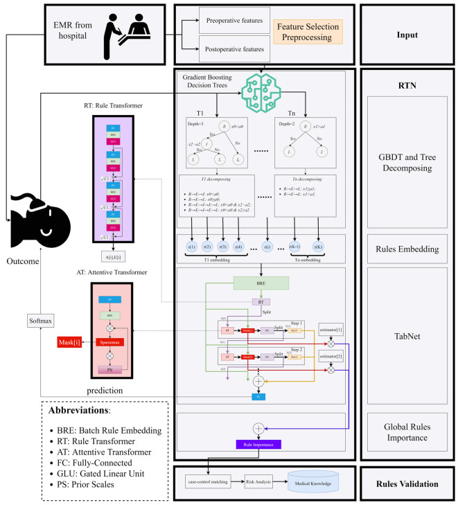
Craniotomy is an invasive operation with great trauma and many complications, and patients undergoing craniotomy should enter the ICU for monitoring and treatment. Based on electronic medical records (EMR), the discovery of high-risk multi-biomarkers rather than a single biomarker that may affect the length of ICU stay (LoICUS) can provide better decision-making or intervention suggestions for clinicians in ICU to reduce the high medical expenses of these patients and the medical burden as much as possible. The multi-biomarkers or medical decision rules can be discovered according to some interpretable predictive models, such as tree-based methods. Our study aimed to develop an interpretable framework based on real-world EMRs to predict the LoICUS and discover some high-risk medical rules of patients undergoing craniotomy. The EMR datasets of patients undergoing craniotomy in ICU were separated into preoperative and postoperative features. The paper proposes a framework called Rules-TabNet (RTN) based on the datasets. RTN is a rule-based classification model. High-risk medical rules can be discovered from RTN, and a risk analysis process is implemented to validate the rules discovered by RTN. The performance of the postoperative model was considerably better than that of the preoperative model. The postoperative RTN model had a better performance compared with the baseline model and achieved an accuracy of 0.76 and an AUC of 0.85 for the task. Twenty-four key decision rules that may have impact on the LoICUS of patients undergoing craniotomy are discovered and validated by our framework. The proposed postoperative RTN model in our framework can precisely predict whether the patients undergoing craniotomy are hospitalized for too long (more than 15 days) in the ICU. We also discovered and validated some key medical decision rules from our framework.

References

[1]	C. L. Beauregard, W. A. Friedman, Routine use of postoperative ICU care for elective craniotomy: a cost-benefit analysis, Surg. Neurol., 60 (2003), 483–489. http://doi.org/10.1016/s0090-3019(03)00517-2 doi: 10.1016/S0090-3019(03)00517-2
[2]	C. Li, L. Chen, J. Feng, D. Wu, W. Xu, Prediction of length of stay on the intensive care unit based on least absolute shrinkage and selection operator, IEEE Access, 7 (2019), 110710–110721. http://doi.org/10.1109/ACCESS.2019.2934166 doi: 10.1109/ACCESS.2019.2934166
[3]	D. Dahl, G. G. Wojtal, M. J. Breslow, R. Holl, D. Huguez, D. Stone, et al., The high cost of low-acuity ICU outliers, J. Healthcare Manage., 57 (2012), 421–433. doi: 10.1097/00115514-201211000-00009
[4]	S. Rose, Mortality risk score prediction in an elderly population using machine learning, Am. J. Epidemiol., 177 (2013), 443–452. http://doi.org/10.1093/aje/kws241 doi: 10.1093/aje/kws241
[5]	B. P. Nguyen, H. N. Pham, H. Tran, N. Nghiem, Q. H. Nguyen, T. T. T. Do, et al., Predicting the onset of type 2 diabetes using wide and deep learning with electronic health records, Comput. Methods Programs Biomed., 182 (2019), 105055. https://doi.org/10.1016/j.cmpb.2019.105055 doi: 10.1016/j.cmpb.2019.105055
[6]	A. H. T. Chia, M. S. Khoo, A. Z. Lim, K. E. Ong, Y. Sun, B. P. Nguyen, et al., Explainable machine learning prediction of ICU mortality, Inf. Med. Unlocked, 25 (2021), 100674. https://doi.org/10.1016/j.imu.2021.100674 doi: 10.1016/j.imu.2021.100674
[7]	T. Gentimis, A. J. Alnaser, A. Durante, K. Cook, R. Steele, Predicting hospital length of stay using neural networks on MIMIC Ⅲ data, in 2017 IEEE 15th Intl Conf on Dependable, Autonomic and Secure Computing, 15th Intl Conf on Pervasive Intelligence and Computing, 3rd Intl Conf on Big Data Intelligence and Computing and Cyber Science and Technology Congress, 2017. http://doi.org/10.1109/DASC-PICom-DataCom-CyberSciTec.2017.191
[8]	H. Harutyunyan, H. Khachatrian, D. C. Kale, G. V. Steeg, A. Galstyan, Multitask learning and benchmarking with clinical time series data, Sci. Data, 6 (2019), 96. http://doi.org/10.1038/s41597-019-0103-9 doi: 10.1038/s41597-019-0103-9
[9]	K. Alghatani, N. Ammar, A. Rezgui, A. Shaban-Nejad, Predicting intensive care unit length of stay and mortality using patient vital signs: machine learning model development and validation, JMIR. Med. Inf., 9 (2021), e21347. http://doi.org/10.2196/21347 doi: 10.2196/21347
[10]	T. Miller, Explanation in artificial intelligence: Insights from the social sciences, Artif. Intell., 267 (2019), 1–38. http://doi.org/10.1016/j.artint.2018.07.007 doi: 10.1016/j.artint.2018.07.007
[11]	T. Chen, C. Guestrin, Xgboost: A scalable tree boosting system, in Proceedings of the 22nd ACM SIGKDD International Conference on Knowledge Discovery and Data Mining, (2016), 13–17. http://doi.org/10.1145/2939672.2939785
[12]	G. Ke, Q. Meng, T. Finley, T. Wang, W. Chen, W. Ma, et al., Lightgbm: A highly efficient gradient boosting decision tree, in Proceedings of the 31st International Conference on Neural Information Processing Systems, (2017), 4–9.
[13]	B. G. Demissei, G. Cotter, M. F. Prescott, G. M. Felker, G. Filippatos, B. H. Greenberg, et al., A multimarker multi-time point based risk stratification strategy in acute heart failure: results from the RELAXAHF trial, Eur. J. Heart Fail., 19 (2017), 1001–1010. http://doi.org/10.1002/ejhf.749 doi: 10.1002/ejhf.749
[14]	S. O. Arik, T. Pfister, TabNet: Attentive interpretable tabular learning, preprint, arXiv: 1908.07442. https://doi.org/10.48550/arXiv.1908.07442
[15]	R. Yu, S. Wang, J. Xu, Q. Wang, X. He, J. Li, et al., Machine learning approaches-driven for mortality prediction for patients undergoing craniotomy in ICU, Brain Inj., 35 (2021), 1658–1664. https://doi.org/10.1080/02699052.2021.2008491 doi: 10.1080/02699052.2021.2008491
[16]	J. H. Friedman, B. E. Popescu, Predictive learning via rule ensembles, Ann. Appl. Stat., 2 (2008), 916–954. http://doi.org/10.1214/07-AOAS148 doi: 10.1214/07-AOAS148
[17]	S. Wang, G. Liu, W. Zhu, Z. Jiao, H. Lv, J. Yan, et al., Interpretable knowledge mining for heart failure prognosis risk evaluation, SEDAMI, (2021), 3032.
[18]	Y. N. Dauphin, A. Fan, M. Auli, D. Grangier, Language modeling with gated convolutional networks, preprint, arXiv: 1612.08083. https://doi.org/10.48550/arXiv.1612.08083
[19]	J. Gehring, M. Auli, D. Grangier, D. Yarats, Y. N. Dauphin, Convolutional Sequence to Sequence Learning, preprint, arXiv: 1705.03122. https://doi.org/10.48550/arXiv.1705.03122
[20]	A. Martins, R. Astudillo, From softmax to sparsemax: A sparse model of attention and multi-label classification, preprint, arXiv: 1602.02068. https://doi.org/10.48550/arXiv.1602.02068
[21]	P. Yadav, M. Steinbach, V. Kumar, G. Simon, Mining electronic health records (EHRs) A survey, ACM Comput. Surv. (CSUR), 50 (2018), 1–40. http://doi.org/10.1145/3127881 doi: 10.1145/3127881
[22]	D. N. Peikes, L. Moreno, S. M. Orzol, Propensity score matching: A note of caution for evaluators of social programs, Am. Stat., 62 (2008), 222–231. http://doi.org/10.1198/000313008X332016 doi: 10.1198/000313008X332016
[23]	A. Thavaneswaran, L. Lix, Propensity score matching in observational studies, Manit. Cent. Health Policy, 2008.
[24]	S. Missios, P. Kalakoti, A. Nanda, K. Bekelis, Craniotomy for glioma resection: a predictive model, World Neurosurg., 83 (2015), 957–964. http://doi.org/10.1016/j.wneu.2015.04.052 doi: 10.1016/j.wneu.2015.04.052
[25]	N. J. Goel, A. N. Mallela, P. Agarwal, K. G. Abdullah, O. A. Choudhri, D. K. Kung, et al., Complications predicting perioperative mortality in patients undergoing elective craniotomy: a population-based study, World Neurosurg., 118 (2018), e195–e205. http://doi.org/10.1016/j.wneu.2018.06.153 doi: 10.1016/j.wneu.2018.06.153
[26]	M. Saeed, M. Saliaj, M. Khan, S. Kumar, Z. Khan, M. Bachan, Isolated elevation of serum alkaline phosphatase in ICU patients, Chest, 154 (2018), 370A. https://doi.org/10.1016/j.chest.2018.08.338 doi: 10.1016/j.chest.2018.08.338
[27]	E. C. Vamvakas, J. H. Carven, RBC transfusion and postoperative length of stay in the hospital or the intensive care unit among patients undergoing coronary artery bypass graft surgery: the effects of confounding factors, Transfusion, 40 (2000), 832–839. https://doi.org/10.1046/j.1537-2995.2000.40070832.x doi: 10.1046/j.1537-2995.2000.40070832.x
[28]	S. Kimura, T. Iwasaki, K. Oe, K. Shimizu, T. Suemori, T. Kanazawa, et al., High ionized calcium concentration is associated with prolonged length of stay in the intensive care unit for postoperative pediatric cardiac patients, J. Cardiothorac. Vasc. Anesth., 32 (2018), 1667–1675. https://doi.org/10.1053/j.jvca.2017.11.006 doi: 10.1053/j.jvca.2017.11.006
[29]	N. Shinoura, R. Yamada, K. Okamoto, O. Nakamura, Early prediction of infection after craniotomy for brain tumours, Br. J. Neurosurg., 18 (2004), 598–603. https://doi.org/10.1080/02688690400022771 doi: 10.1080/02688690400022771
[30]	H. Wang, Higher Procalcitonin level in cerebrospinal fluid than in serum is a feasible Indicator for diagnosis of intracranial infection, Surg. Infect., 21 (2020), 704–708. http://doi.org/10.1089/sur.2019.194 doi: 10.1089/sur.2019.194
[31]	A. B. Böhmer, K. S. Just, R. Lefering, T. Paffrath, B, Bouillon. R. Joppich, et al., Factors influencing lengths of stay in the intensive care unit for surviving trauma patients: A retrospective analysis of 30,157 cases, Crit. Care., 18 (2014), 1–10. https://doi.org/10.1186/cc13976 doi: 10.1186/cc13976
[32]	Z. Zhang, X. Xu, H. Ni, H. Deng, Urine output on ICU entry is associated with hospital mortality in unselected critically ill patients, J. Nephrol., 27 (2014), 65–71. http://doi.org/10.1007/s40620-013-0024-1 doi: 10.1007/s40620-013-0024-1
[33]	M. Nagae, M. Egi, K. Kubota, S. Makino, S. Mizobuchi, Association of direct bilirubin level with postoperative outcome in critically ill postoperative patients, Korean J. Anesthesiol., 71 (2018), 30–36. https://doi.org/10.4097/kjae.2018.71.1.30 doi: 10.4097/kjae.2018.71.1.30
[34]	M. Zhang, Y. Chen, J. Lin, A privacy-preserving optimization of neighborhood-based recommendation for medical-aided diagnosis and treatment, IEEE Internet Things J., 8 (2021), 10830–10842. http://doi.org/10.1109/JIOT.2021.3051060 doi: 10.1109/JIOT.2021.3051060
[35]	C. Li, M. Dong, J. Li, G. Xu, X. Chen, W. Liu, et al., Efficient medical big data management with keyword-searchable encryption in healthchain, IEEE Syst. J., 2022. http://doi.org/10.1109/JSYST.2022.3173538 doi: 10.1109/JSYST.2022.3173538
[36]	L. Grinsztajn, E. Oyallon, G. Varoquaux, Why do tree-based models still outperform deep learning on tabular data, preprint, arXiv: 2207.08815. https://doi.org/10.48550/arXiv.2207.08815
[37]	B. P. Nguyen, W. L. Tay, C. K. Chui, Robust biometric recognition from palm depth images for gloved hands, IEEE Trans. Human Mach. Syst., 45 (2015), 799–804. http://doi.org/10.1109/THMS.2015.2453203 doi: 10.1109/THMS.2015.2453203
[38]	J. C. Ferrão, F. Janela, M. D. Oliveira, H. M. G. Martins, Using structured EHR data and SVM to support ICD-9-CM coding, in 2013 IEEE International Conference on Healthcare Informatics, (2013), 511–516. http://doi.org/10.1109/ICHI.2013.79

mbe-20-01-038-supplementary.docx

Reader Comments

Your name:*

Email:*
© 2023 the Author(s), licensee AIMS Press. This is an open access article distributed under the terms of the Creative Commons Attribution License (http://creativecommons.org/licenses/by/4.0)