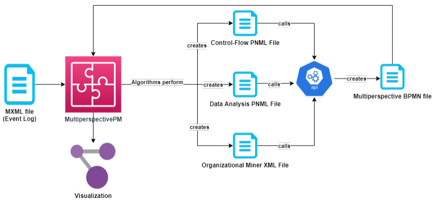
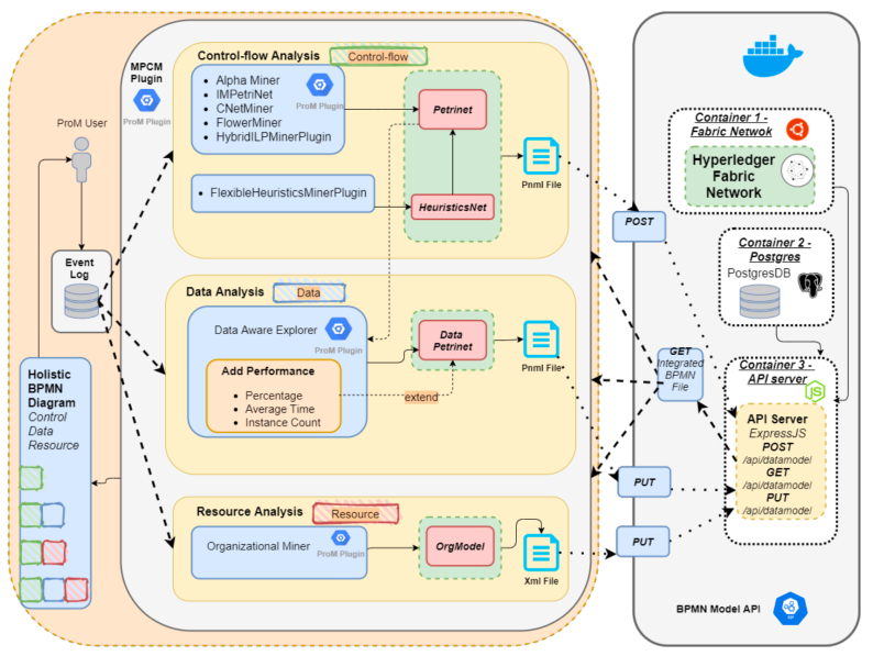
Process mining is mainly focused on process discovery from control perspective. It is further applied to mine the other perspectives such as time, data, and resources by replaying the events in event logs over the initial process model. When process mining is extended far beyond discovering the control-flow models to capture additional perspectives; roles, bottlenecks, amounts of time passed, guards, and routing probabilities in the process can be identified. This is a such extensions are considered under the topic of multi-perspective process mining, which makes the discovered process model more understandable. In this study, a framework for applying multi-perspective process mining and creating a Business Process Modelling Notation (BPMN) process model as the output is introduced. The framework, which uses a recently developed application programming interface (API) for storing the BPMN Data Model which keeps what is produced from each perspective as an asset into a private blockchain in a secure and immutable way, has been developed as a plugin to the ProM tool. In doing so, it integrates a number of techniques for multi-perspective process mining in literature, for the perspectives of control-flow, data, and resource; and represents a holistic process model by combining the outputs of these in the BPMN Data Model. In this article, we explain technical details of the framework and also demonstrate its usage over a case in medical domain.
Citation: Merve Nur TİFTİK, Tugba GURGEN ERDOGAN, Ayça KOLUKISA TARHAN. A framework for multi-perspective process mining into a BPMN process model[J]. Mathematical Biosciences and Engineering, 2022, 19(11): 11800-11820. doi: 10.3934/mbe.2022550
Process mining is mainly focused on process discovery from control perspective. It is further applied to mine the other perspectives such as time, data, and resources by replaying the events in event logs over the initial process model. When process mining is extended far beyond discovering the control-flow models to capture additional perspectives; roles, bottlenecks, amounts of time passed, guards, and routing probabilities in the process can be identified. This is a such extensions are considered under the topic of multi-perspective process mining, which makes the discovered process model more understandable. In this study, a framework for applying multi-perspective process mining and creating a Business Process Modelling Notation (BPMN) process model as the output is introduced. The framework, which uses a recently developed application programming interface (API) for storing the BPMN Data Model which keeps what is produced from each perspective as an asset into a private blockchain in a secure and immutable way, has been developed as a plugin to the ProM tool. In doing so, it integrates a number of techniques for multi-perspective process mining in literature, for the perspectives of control-flow, data, and resource; and represents a holistic process model by combining the outputs of these in the BPMN Data Model. In this article, we explain technical details of the framework and also demonstrate its usage over a case in medical domain.

| [1] | M. Dumas, M. La Rosa, J. Mendling, H. A. Reijers, Fundamentals of business process management, Springer, (2013). https://doi.org/10.1007/978-3-642-33143-5 |
| [2] | A. J. M. M Weijters, W. M. van Der Aalst, A. A. De Medeiros, Process mining with the heuristics miner-algorithm, Technische Universiteit Eindhoven Tech. Rep. WP, 166 (2006), 1–34. |
| [3] |
M. De Leoni, W. M. van der Aalst, M. Dees, A general process mining framework for correlating, predicting and clustering dynamic behavior based on event logs, Inform. Syst., 56 (2016), 235–257. https://doi.org/10.1016/j.is.2015.07.003 doi: 10.1016/j.is.2015.07.003

|
| [4] | F. Mannhardt, Multi-perspective process mining, BPM (Dissertation/Demos/Industry), (2018). |
| [5] | J. L. Peterson, Petri net theory and the modeling of systems, Prentice Hall PTR, (1981). |
| [6] |
R. M. Dijkman, M. Dumas, C. Ouyan, Semantics and analysis of business process models in BPMN, Inform. Software Technol., 50 (2008), 1281–1294. https://doi.org/10.1016/j.infsof.2008.02.006 doi: 10.1016/j.infsof.2008.02.006
|
| [7] | J. M. Colom, J. Desel, Application and theory of petri nets and concurrency, Springer, Italy, 2013. https://doi.org/10.1007/978-3-319-19488-2 |
| [8] | W. M. Van der Aalst, B. F. van Dongen, C. W. Günther, A. Rozinat, E. Verbeek, T. Weijters, ProM: The process mining toolkit, BPM (Demos), 489 (2009). |
| [9] | B. Ekici, A BPMN data model to keep a multi-perspective process model on the blockchain, Fen Bilimleri Enstitüsü, Hacettepe University in Turkey, 2021. |
| [10] | B. Ekici, T. G. Erdogan, A. K. Tarhan, BPMN data model for multi-perspective process mining on blockchain, Int. J. Software Eng. Knowl. Eng., (2022), 1–29. https://doi.org/10.1142/S0218194022500115 |
| [11] |
T. G. Erdogan, A. K. Tarhan, Multi-perspective process mining for emergency process, Health Inform. J., 28 (2022), 14604582221077195. https://doi.org/10.1177/14604582221077195 doi: 10.1177/14604582221077195
|
| [12] | W. Van Der Aalst, Process mining: Data science in action, Springer, (2016). https://doi.org/10.1007/978-3-662-49851-4_1 |
| [13] | W. V. D. Aalst, A. Adriansyah, A. K. A. D. Medeiros, F. Arcieri, T. Baier, T. Blickle, et al., Process mining manifesto, in Springer, International conference on business process management, (2011), 169–194. https://doi.org/10.1007/978-3-642-28108-2_19 |
| [14] |
M. Rovani, F. M. Maggiand, M. De Leoni, W. M. Van Der Aalst, Declarative process mining in healthcare, Expert Syst. Appl., 42 (2015), 9236–9251. https://doi.org/10.1016/j.eswa.2015.07.040 doi: 10.1016/j.eswa.2015.07.040
|
| [15] |
W. Van der Aalst, T. Weijters, L. Maruster, Workflow mining: Discovering process models from event logs, IEEE Transact. Knowl. Data Eng., 16 (2004), 1128–1142. https://doi.org/10.1109/TKDE.2004.47 doi: 10.1109/TKDE.2004.47
|
| [16] | M. De Leoni, W. M. van der Aalst, Data-aware process mining: discovering decisions in processes using alignments, in Proceedings of the 28th annual ACM symposium on applied computing, (2013), 1454–1461. https://doi.org/10.1145/2480362.2480633 |
| [17] | S. J. Leemans, D. Fahland, W. M. Van Der Aalst, Process and deviation exploration with inductive visual miner, BPM (demos), 1295 (2014). |
| [18] | A. A. F. G. Mohamed, Process mining application considering the organizational perspective using social network analysis, University of Porto, 2016. |
| [19] | M. Song, W. M. van der Aalst, Supporting process mining by showing events at a glance, in Proceedings of the 17th Annual Workshop on Information Technologies and Systems (WITS), (2007), 139–145. |
| [20] | F. Mannhardt, M. De Leoni, H. A. Reijers, The multi-perspective process explorer, BPM (Demos), 1418 (2015), 130–134. |
| [21] |
T. G. Erdogan, A. Tarhan, Systematic mapping of process mining studies in healthcare, IEEE Access, 6 (2018), 24543–24567. https://doi.org/10.1109/ACCESS.2018.2831244 doi: 10.1109/ACCESS.2018.2831244
|
| [22] | A. Rozinat, C. W. Günther, R. Niks, Process mining and automated process discovery software for professionals-Fluxicon Disco, (2017). |
| [23] | E. Rojas, C. Fernández-Llatas, V. Traver, V. Munoz-Gama, M. Sepúlveda, V. Herskovic et al., PALIA-ER: Bringing question-driven process mining closer to the emergency room, in BPM (Demos), (2017). |
| [24] | Process Mining and Execution Management Software, Celonis, 2022. Available from: https://www.celonis.com/. |
| [25] | R. Gatta, J. Lenkowicz, M. Vallati, E. Rojas, A. Damiani, L. Sacchi, et al., pMineR: An innovative R library for performing process mining in medicine, in Conference on artificial intelligence in medicine in europe, (2017), 351–355. https://doi.org/10.1007/978-3-319-59758-4_42 |
| [26] |
G. Janssenswillen, B. Depaire, M. Swennen, M. Jans, K. Vanhoof, bupaR: Enabling reproducible business process analysis, Knowledge-Based Syst., 163 (2019), 927–930. https://doi.org/10.1016/j.knosys.2018.10.018 doi: 10.1016/j.knosys.2018.10.018
|
| [27] | U. Celik, E. Akcetin Surec madenciligi araclari karsilastirmasi AJIT-e: Bilişim Teknolojileri Online Dergisi, 9 (2018), 97–104. https://doi.org/10.5824/1309-1581.2018.4.007.x |
| [28] |
D. Dakic, D. Stefanovic, I. Cosic, T. Lolic, M. Medojevic, Business process mining application: A literature review, Ann. DAAAM Proceed., 29 (2018). https://doi.org/10.2507/29th.daaam.proceedings.125 doi: 10.2507/29th.daaam.proceedings.125
|
| [29] | A. Kalenkova, A. Burattin, M. de Leoni, W. van der Aalst, A. Sperduti, Discovering high-level BPMN process models from event data, Business Process Manag. J., (2019). https://doi.org/10.1108/BPMJ-02-2018-0051 |
| [30] | D. Bell, UML basics: An introduction to the Unified Modeling Language, Rational Edge, (2003). |
| [31] |
J. Mendling, M. Nüttgens, EPC markup language (EPML): An XML-based interchange format for event-driven process chains (EPC), Inform. Syst. E-business Manag., 4 (2006), 245–263. https://doi.org/10.1007/s10257-005-0026-1 doi: 10.1007/s10257-005-0026-1
|
| [32] |
M. Geiger, S. Harrer, J. Lenhard, G. Wirtz, BPMN 2.0: The state of support and implementation, Future Gener. Computer Syst., 80 (2018), 250–262. https://doi.org/10.1016/j.future.2017.01.006 doi: 10.1016/j.future.2017.01.006
|
| [33] | J. C. Buijs, B. F. V. Dongen, W.M van Der Aalst, On the role of fitness, precision, generalization and simplicity in process discovery, in OTM Confederated International Conferences" On the Move to Meaningful Internet Systems", (2012), 305–322. https://doi.org/10.1007/978-3-642-33606-5_19 |
| [34] | J. Carmona Vargas, J. Cortadella, M. Kishinevsky, Region-based algorithms for process mining and synthesis of Petri nets, Polytechnic University of Catalonia, (2009). |
| [35] | R. Bergenthum, J. Desel, R. Lorenz, S. Mauser, Process mining based on regions of languages, in International Conference on Business Process Management, (2007), 375–383. https://doi.org/10.1007/978-3-540-75183-0_27 |
| [36] | J. M. E. Van der Werf, B. F. van Dongen, C. A. Hurkens, A. Serebrenik, Process discovery using integer linear programming, in International conference on applications and theory of petri nets, (2008), 368–387 https://doi.org/10.1007/978-3-540-68746-7_24 |
| [37] | C. W. Günther, W. M. Van Der Aalst, Fuzzy mining–adaptive process simplification based on multi-perspective metrics, in International conference on business process management, (2007), 328–343. https://doi.org/10.1007/978-3-540-75183-0_24 |
| [38] | W. M. van der Aalst, On the representational bias in process mining, in 2011 IEEE 20th International Workshops on Enabling Technologies: Infrastructure for Collaborative Enterprises, (2011), 2–7. https://doi.org/10.1109/WETICE.2011.64 |
| [39] | W. M. Van der Aalst, A. K. De Medeiros, A. J. Weijters, Genetic process mining, in International conference on application and theory of petri nets, (2005), 48–69. https://doi.org/10.1007/11494744_5 |
| [40] | P. Weber, B. Bordbar, P. Tiňo, A principled approach to the analysis of process mining algorithms, in International Conference on Intelligent Data Engineering and Automated Learning, (2011), 474–481. https://doi.org/10.1007/978-3-642-23878-9_56 |
| [41] | R. Ghawi, Process discovery using inductive miner and decomposition, arXiv preprint arXiv: 1610.07989, (2016). |
| [42] | A. Rozinat, W. M. van der Aalst, Decision mining in ProM, in International Conference on Business Process Management, (2006), 420–425. https://doi.org/10.1007/11841760_33 |
| [43] | R. S. Mans, M. H. Schonenberg, M. Song, W. M. van der Aalst, P. J. Bakker, Application of process mining in healthcare–a case study in a dutch hospital, in International joint conference on biomedical engineering systems and technologies, (2008), 425–438. https://doi.org/10.1007/978-3-540-92219-3_32 |
| [44] | M. Bozkaya, J. Gabriels, J. M. van der Werf, Process diagnostics: A method based on process mining, in International Conference on Information, Process, and Knowledge Management, 1 (2009), 22–27. https://doi.org/10.1109/eKNOW.2009.29 |
| [45] |
W. Van Der Aalst, Service mining: Using process mining to discover, check, and improve service behavior, IEEE Transact. Services Comput., 6 (2012), 525–535. https://doi.org/10.1109/TSC.2012.25 doi: 10.1109/TSC.2012.25
|
| [46] | E. Gupta, Process mining algorithms, Int. J. Adv. Res. Sci. Eng., 3 (2014), 401–412. |
| [47] | F. Folino, G. Greco, A. Guzzo, L. Pontieri, Discovering multi-perspective process models: The case of loosely-structured processes, in International Conference on Enterprise Information Systems, 19 (2008). https://doi.org/10.1007/978-3-642-00670-8_10 |
| [48] | A. Pini, R. Brown, M. T. Wynn, Process visualization techniques for multi-perspective process comparisons, in Asia-Pacific Conference on Business Process Management, (2015), 183–197. https://doi.org/10.1007/978-3-319-19509-4_14 |
| [49] |
S. Schönig, C. D. Ciccio, F. M. Maggi, J. Mendling, Discovery of multi-perspective declarative process models, International Conference on Service-Oriented Computing, 9936 (2016), 87–103. https://doi.org/10.1007/978-3-319-46295-0_6 doi: 10.1007/978-3-319-46295-0_6
|
| [50] |
S. Jablonski, M. Röglinger, S. Schönig, K. M. Wyrtki, Multi-perspective clustering of process execution traces, Enterprise Model. Inform. Syst. Archit. (EMISAJ), 14 (2019), 2–11. https://doi.org/10.18417/emisa.14.2 doi: 10.18417/emisa.14.2
|
| [51] | R. Sikal, H. Sbai, L. Kjiri, Promoting resource discovery in business process variability, in Proceedings of the 2nd International Conference on Networking, Information Systems & Security, (2019), 1–7. https://doi.org/10.1145/3320326.3320380 |
| [52] | C. Sturm, S. Schönig, C. Di Ciccio, Distributed multi-perspective declare discovery, in BPM (Demos), (2017). |
| [53] | Tijs Slaats, Flexible process notations for cross-organizational case management systems, IT University of Copenhagen, Theoretical computer Science section, 2015. |
| [54] | A. J. M. M. Weijters, J. T. S. Ribeiro, Flexible heuristics miner (FHM), in Flexible heuristics miner (FHM), (2011). https://doi.org/10.1109/CIDM.2011.5949453 |
| [55] | W. V. D. Aalst, A. Adriansyah, B. V. Dongen, Causal nets: A modeling language tailored towards process discovery, in International conference on concurrency theory, 6901 (2011), 28–42. https://doi.org/10.1007/978-3-642-23217-6_3 |
| [56] |
V. M. Van der Aalst, V. Rubin, H. M. W. Verbeek, B. F. van Dongen, E. Kindler, C. W. Günther, Process mining: a two-step approach to balance between underfitting and overfitting, Software Syst. Model., 9 (2010), 87–111. https://doi.org/10.1007/s10270-008-0106-z doi: 10.1007/s10270-008-0106-z
|
| [57] | F. Mannhardt, D. Blinde, Analyzing the trajectories of patients with sepsis using process mining, in RADAR+ EMISA@ CAiSE, (2017). |
| [58] |
Á. Rebuge, D. R. Ferreira, Business process analysis in healthcare environments: A methodology based on process mining, Inform. Syst., 37 (2012), 99–116. https://doi.org/10.1016/j.is.2011.01.003 doi: 10.1016/j.is.2011.01.003
|
| [59] | ProM 6.10, Accessed on 31.12.2021. Available from: http://www.promtools.org/doku.php?id=prom610. |
Figures(10) / Tables(4)

Merve Nur TİFTİK, Tugba GURGEN ERDOGAN, Ayça KOLUKISA TARHAN. A framework for multi-perspective process mining into a BPMN process model[J]. Mathematical Biosciences and Engineering, 2022, 19(11): 11800-11820. doi: 10.3934/mbe.2022550


 DownLoad: