This paper proposes a probabilistic graphical model that integrates interpretive structural modeling (ISM) and Bayesian belief network (BBN) approaches to predict cone penetration test (CPT)-based soil liquefaction potential. In this study, an ISM approach was employed to identify relationships between influence factors, whereas BBN approach was used to describe the quantitative strength of their relationships using conditional and marginal probabilities. The proposed model combines major causes, such as soil, seismic and site conditions, of seismic soil liquefaction at once. To demonstrate the application of the propose framework, the paper elaborates on each phase of the BBN framework, which is then validated with historical empirical data. In context of the rate of successful prediction of liquefaction and non-liquefaction events, the proposed probabilistic graphical model is proven to be more effective, compared to logistic regression, support vector machine, random forest and naive Bayes methods. This research also interprets sensitivity analysis and the most probable explanation of seismic soil liquefaction appertaining to engineering perspective.
Citation: Mahmood Ahmad, Feezan Ahmad, Jiandong Huang, Muhammad Junaid Iqbal, Muhammad Safdar, Nima Pirhadi. Probabilistic evaluation of CPT-based seismic soil liquefaction potential: towards the integration of interpretive structural modeling and bayesian belief network[J]. Mathematical Biosciences and Engineering, 2021, 18(6): 9233-9252. doi: 10.3934/mbe.2021454
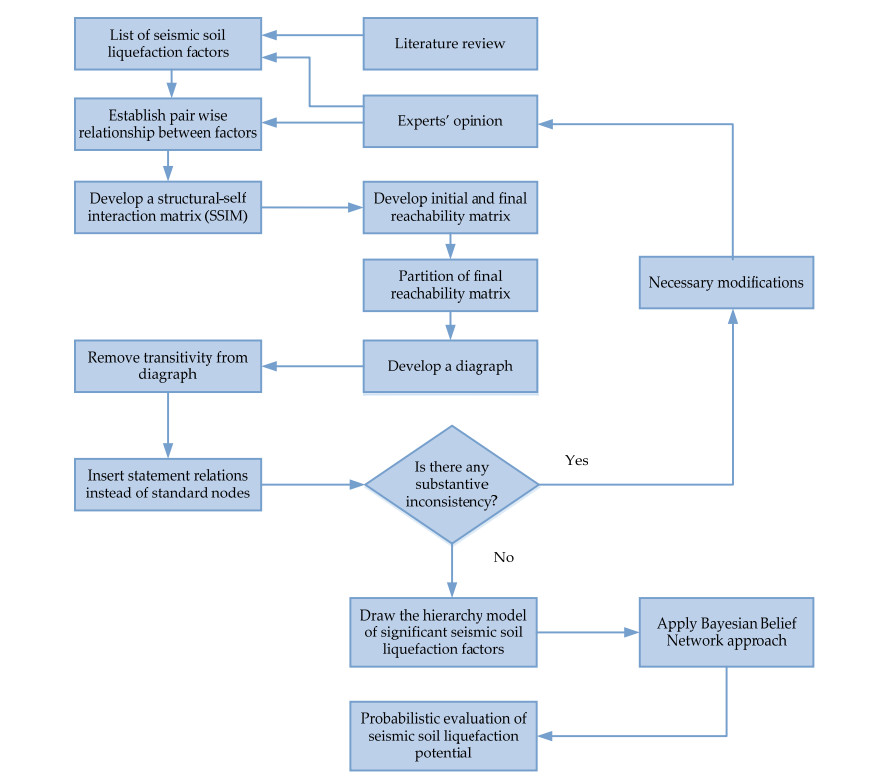
This paper proposes a probabilistic graphical model that integrates interpretive structural modeling (ISM) and Bayesian belief network (BBN) approaches to predict cone penetration test (CPT)-based soil liquefaction potential. In this study, an ISM approach was employed to identify relationships between influence factors, whereas BBN approach was used to describe the quantitative strength of their relationships using conditional and marginal probabilities. The proposed model combines major causes, such as soil, seismic and site conditions, of seismic soil liquefaction at once. To demonstrate the application of the propose framework, the paper elaborates on each phase of the BBN framework, which is then validated with historical empirical data. In context of the rate of successful prediction of liquefaction and non-liquefaction events, the proposed probabilistic graphical model is proven to be more effective, compared to logistic regression, support vector machine, random forest and naive Bayes methods. This research also interprets sensitivity analysis and the most probable explanation of seismic soil liquefaction appertaining to engineering perspective.

| [1] |
H. B. Seed, I. M. Idriss, Simplified procedure for evaluating soil liquefaction potential, J. Soil Mech. Found. Div., 97 (1971), 1249-1273. doi: 10.1061/JSFEAQ.0001662

|
| [2] | H. B. Seed, I. M. Idriss, Evaluation of liquefaction potential sand deposits based on observation of performance in previous earthquakes, in Proceedings of ASCE national convention (MO), 481-544. |
| [3] |
P. K. Robertson, C. Wride, Evaluating cyclic liquefaction potential using the cone penetration test, Can. Geotech. J., 35 (1998), 442-459. doi: 10.1139/t98-017
|
| [4] |
T. L. Youd, I. M. Idriss, Liquefaction resistance of soils: summary report from the 1996 NCEER and 1998 NCEER/NSF workshops on evaluation of liquefaction resistance of soils, J. Geotech. Geoenviron., 127 (2001), 297-313. doi: 10.1061/(ASCE)1090-0241(2001)127:4(297)
|
| [5] |
C. H. Juang, H. Yuan, D. H. Lee, P. S. Lin, Simplified cone penetration test-based method for evaluating liquefaction resistance of soils, J. Geotech. Geoenviron., 129 (2003), 66-80. doi: 10.1061/(ASCE)1090-0241(2003)129:1(66)
|
| [6] |
R. Moss, R. B. Seed, R. E. Kayen, J. P. Stewart, A. Der Kiureghian, K. O. Cetin, CPT-based probabilistic and deterministic assessment of in situ seismic soil liquefaction potential, J. Geotech. Geoenviron., 132 (2006), 1032-1051. doi: 10.1061/(ASCE)1090-0241(2006)132:8(1032)
|
| [7] |
I. Idriss, R. Boulanger, Semi-empirical procedures for evaluating liquefaction potential during earthquakes, Soil Dyn. Earthquake Eng., 26 (2006), 115-130. doi: 10.1016/j.soildyn.2004.11.023
|
| [8] |
V. Kohestani, M. Hassanlourad, A. Ardakani, Evaluation of liquefaction potential based on CPT data using random forest, Nat. Hazards, 79 (2015), 1079-1089. doi: 10.1007/s11069-015-1893-5
|
| [9] |
X. Xue, X. Yang, Application of the adaptive neuro-fuzzy inference system for prediction of soil liquefaction, Nat. Hazards, 67 (2013), 901-917. doi: 10.1007/s11069-013-0615-0
|
| [10] |
P. Samui, Seismic liquefaction potential assessment by using relevance vector machine, Earthquake Eng. Eng. Vib., 6 (2007), 331-336. doi: 10.1007/s11803-007-0766-7
|
| [11] |
A. T. Goh, Neural-network modeling of CPT seismic liquefaction data, J. Geotech. Eng., 122 (1996), 70-73. doi: 10.1061/(ASCE)0733-9410(1996)122:1(70)
|
| [12] |
P. Samui, T. Sitharam, M. Contadakis, Machine learning modelling for predicting soil liquefaction susceptibility, Nat. Hazards Earth Syst. Sci., 11 (2011), 1-9. doi: 10.5194/nhess-11-1-2011
|
| [13] |
A. H. Gandomi, A. H. Alavi, A new multi-gene genetic programming approach to non-linear system modeling. Part Ⅱ: geotechnical and earthquake engineering problems, Neural Comput. Appl., 21 (2012), 189-201. doi: 10.1007/s00521-011-0735-y
|
| [14] |
P. K. Muduli, S. K. Das, CPT-based seismic liquefaction potential evaluation using multi-gene genetic programming approach, Indian Geotech. J., 44 (2014), 86-93. doi: 10.1007/s40098-013-0048-4
|
| [15] |
P. K. Muduli, S. K. Das, S. Bhattacharya, CPT-based probabilistic evaluation of seismic soil liquefaction potential using multi-gene genetic programming, Georisk: Assess. Manage. Risk Eng. Syst. Geohazards, 8 (2014), 14-28. doi: 10.1080/17499518.2013.845720
|
| [16] |
P. K. Muduli, S. K. Das, First-order reliability method for probabilistic evaluation of liquefaction potential of soil using genetic programming, Int. J. Geomech., 15 (2015), 04014052. doi: 10.1061/(ASCE)GM.1943-5622.0000377
|
| [17] |
A. T. Goh, S. Goh, Support vector machines: their use in geotechnical engineering as illustrated using seismic liquefaction data, Comput. Geotech., 34 (2007), 410-421. doi: 10.1016/j.compgeo.2007.06.001
|
| [18] |
T. Oommen, L. G. Baise, R. Vogel, Validation and application of empirical liquefaction models, J. Geotech. Geoenviron., 136 (2010), 1618-1633. doi: 10.1061/(ASCE)GT.1943-5606.0000395
|
| [19] |
M. Pal, Support vector machines-based modelling of seismic liquefaction potential, Int. J. Numer. Anal. Methods Geomech., 30 (2006), 983-996. doi: 10.1002/nag.509
|
| [20] | J. Pearl, Probabilistic reasoning in intelligent systems: Representation & reasoning, Morgan Kaufmann Publishers, San Mateo, 1988. |
| [21] |
M. Ahmad, X. W. Tang, J. N. Qiu, W. J. Gu, F. Ahmad, A hybrid approach for evaluating CPT-based seismic soil liquefaction potential using Bayesian belief networks, J. Cent. South Univ., 27 (2020), 500-516. doi: 10.1007/s11771-020-4312-3
|
| [22] |
M. Ahmad, X. W. Tang, J. N. Qiu, F. Ahmad, W. J. Gu, A step forward towards a comprehensive framework for assessing liquefaction land damage vulnerability: Exploration from historical data, Front. Struct. Civ. Eng., 14 (2020), 1476-1491. doi: 10.1007/s11709-020-0670-z
|
| [23] |
M. Ahmad, X. W. Tang, J. N. Qiu, F. Ahmad, Evaluating Seismic Soil Liquefaction Potential Using Bayesian Belief Network and C4. 5 Decision Tree Approaches, Appl. Sci., 9 (2019), 4226. doi: 10.3390/app9204226
|
| [24] | A. P. Sage, Methodology for Large-Scale Systems, New York, 1977. |
| [25] | J. N. Warfield, Developing interconnection matrices in structural modeling, IEEE Trans. Syst. Man Cybern., 4 (1974), 81-87. |
| [26] |
V. Ravi, R. Shankar, Analysis of interactions among the barriers of reverse logistics, Technol. Forecast. Soc. Change., 72 (2005), 1011-1029. doi: 10.1016/j.techfore.2004.07.002
|
| [27] |
R. Shankar, R. Narain, A. Agarwal, An interpretive structural modeling of knowledge management in engineering industries, J. Adv. Manag. Res., 1 (2003), 28-40. doi: 10.1108/97279810380000356
|
| [28] |
T. Raj, R. Attri, Identification and modelling of barriers in the implementation of TQM, Int. J. Product. Qual., 8 (2011), 153-179. doi: 10.1504/IJPQM.2011.041844
|
| [29] |
M. Ahmad, X. W. Tang, J. N. Qiu, F. Ahmad, Evaluation of liquefaction-induced lateral displacement using Bayesian belief networks, Front. Struct. Civ. Eng., 15 (2021), 80-98, doi: 10.1007/s11709-021-0682-3
|
| [30] | M. Ahmad, X. W. Tang, F. Ahmad, M. Hadzima-Nyarko, A. Nawaz, A. Farooq, Elucidation of Seismic Soil Liquefaction Significant Factors. in Earthquakes-From Tectonics to Buildings, 2021. |
| [31] |
K. Masmoudi, L. Abid, A. Masmoudi, Credit risk modeling using Bayesian network with a latent variable, Expert Syst. Appl., 127 (2019), 157-166. doi: 10.1016/j.eswa.2019.03.014
|
| [32] | A. Castelletti, R. Soncini-Sessa, Bayesian Networks and participatory modelling in water resource management, Environ. Model. Software, 22 (2007), 1075-1088. |
| [33] |
A. Ghribi, A. Masmoudi, A compound poisson model for learning discrete Bayesian networks, Acta Math. Sci., 33 (2013), 1767-1784. doi: 10.1016/S0252-9602(13)60122-8
|
| [34] |
S. A. Joseph, B. J. Adams, B. McCabe, Methodology for Bayesian belief network development to facilitate compliance with water quality regulations, J. Infrastruct. Syst., 16 (2010), 58-65. doi: 10.1061/(ASCE)1076-0342(2010)16:1(58)
|
| [35] |
S. Nadkarni, P. P. Shenoy, A Bayesian network approach to making inferences in causal maps, Eur. J. Oper. Res., 128 (2001), 479-498. doi: 10.1016/S0377-2217(99)00368-9
|
| [36] |
G. Kabir, S. Tesfamariam, A. Francisque, R. Sadiq, Evaluating risk of water mains failure using a Bayesian belief network model, Eur. J. Oper. Res., 240 (2015), 220-234. doi: 10.1016/j.ejor.2014.06.033
|
| [37] | S. Tesfamariam, Z. Liu, Seismic risk analysis using Bayesian belief networks, in Handbook of seismic risk analysis and management of civil infrastructure systems, 2013,175-208. |
| [38] | R. Boulanger, I. Idriss, CPT and SPT based liquefaction triggering procedures, 2014. |
| [39] | C. Okoli, K. Schabram, A guide to conducting a systematic literature review of information systems research, Inf. Syst., 10 (2010), 1-51. |
| [40] |
D. Tranfield, D. Denyer, P. Smart, Towards a methodology for developing evidence-informed management knowledge by means of systematic review, Br. J. Manage., 14 (2003), 207-222. doi: 10.1111/1467-8551.00375
|
| [41] |
M. Ahmad, X. W. Tang, J. N. Qiu, F. Ahmad, Interpretive Structural Modeling and MICMAC Analysis for Identifying and Benchmarking Significant Factors of Seismic Soil Liquefaction, Appl. Sci., 9 (2019), 233. doi: 10.3390/app9020233
|
| [42] |
L. Zhang, Predicting seismic liquefaction potential of sands by optimum seeking method, Soil Dyn. Earthquake Eng., 17 (1998), 219-226. doi: 10.1016/S0267-7261(98)00004-9
|
| [43] |
J. L. Hu, X. W. Tang, J. N. Qiu, A Bayesian network approach for predicting seismic liquefaction based on interpretive structural modeling, Georisk: Assess. Manage. Risk Eng. Syst. Geohazards, 9 (2015), 200-217. doi: 10.1080/17499518.2015.1076570
|
| [44] | D. W. Hosmer, S. Lemeshow, Applied Logistic Regression, 2nd edition, John Wiley & Sons, New York, 2000. |
| [45] | V. N. Vapnik, The nature of statistical learning, Theory, 1995. |
| [46] | L. Breiman, Random forests, Mach. Learn., 45 (2001), 5-32. |
| [47] | G. John, P. Langley, Estimating Continuous Distributions in Bayesian Classifiers, in proceedings of the Eleventh Conference on Uncertainty in Artificial Intelligence, 1995. |
| [48] |
S. K. Das, R. Mohanty, M. Mohanty, M. Mahamaya, Multi-objective feature selection (MOFS) algorithms for prediction of liquefaction susceptibility of soil based on in situ test methods, Nat. Hazards, 103 (2020), 2371-2393. doi: 10.1007/s11069-020-04089-3
|
| [49] | M. Kubat, S. Matwin, Addressing the curse of imbalanced training sets: one-sided selection, in Proceedings of the Fourteenth International Conference on Machine Learning, (1997), 179-186. |
| [50] | B. Yuan, W. Liu, A measure oriented training scheme for imbalanced classification problems, in Proceedings of Pacific-Asia Conference on Knowledge Discovery and Data Mining, (2001), 293-303. |
| [51] | Y. Sun, M. S. Kamel, Y. Wang, Boosting for learning multiple classes with imbalanced class distribution, in Proceedings of Sixth international conference on data mining (ICDM06), (2006), 592-602. |


Figures(5) / Tables(15)

Mahmood Ahmad, Feezan Ahmad, Jiandong Huang, Muhammad Junaid Iqbal, Muhammad Safdar, Nima Pirhadi. Probabilistic evaluation of CPT-based seismic soil liquefaction potential: towards the integration of interpretive structural modeling and bayesian belief network[J]. Mathematical Biosciences and Engineering, 2021, 18(6): 9233-9252. doi: 10.3934/mbe.2021454


 DownLoad: