Mathematical modeling of impact of eCD4-Ig molecule in control and management of HIV within a host

Tae Jin Lee; Jose A. Vazquez; Arni S. R. Srinivasa Rao; Tae Jin Lee; Jose A. Vazquez; Arni S. R. Srinivasa Rao

doi:10.3934/mbe.2021342

Mathematical Biosciences and Engineering

2021, Volume 18, Issue 5: 6887-6906. doi: 10.3934/mbe.2021342

Previous Article Next Article

Research article Special Issues

Mathematical modeling of impact of eCD4-Ig molecule in control and management of HIV within a host

1.
Center for Biotechnology and Genomic Medicine, Medical College of Georgia, Augusta University, 1120 15th Street, Augusta, GA 30912, USA
2.
Division of Infectious Diseases, Department of Medicine, Medical College of Georgia, Augusta University, 1120 15th Street, Augusta, GA 30912, USA
3.
Laboratory for Theory and Mathematical Modeling, Division of Infectious Diseases, Department of Medicine, Medical College of Georgia, Augusta University, 1120 15th Street, Augusta, GA 30912, USA
4.
Department of Mathematics, Augusta University, 1120 15th Street, Augusta, GA 30912, USA

Received: 18 June 2021 Accepted: 12 August 2021 Published: 19 August 2021

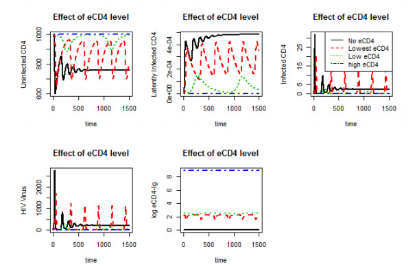
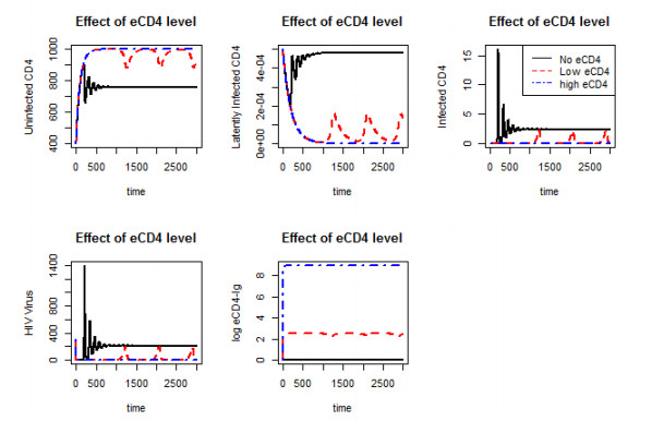
Eradication and eventually cure of the HIV virus from the infected individual should be the primary goal in all HIV therapy. This has yet to be achieved, however development of broadly neutralizing antibodies (bNabs) and eCD4-Ig and its related particles are promising therapeutic alternatives to eliminate the HIV virus from the host. Past studies have found superior protectivity and efficacy eradicating the HIV virus with the use of eCD4-Igs over bNabs, which has proposed the antibody-dependent cell-mediated cytotoxicity (ADCC) effect as one of the key-factors for antibody design. In this study, we evaluated the dynamics of the HIV virus, CD4 T-cells, and eCD4-Ig in humans using a gene-therapy approach which has been evaluated in primates previously. We utilized a mathematical model to investigate the relationship between eCD4-Ig levels, ADCC effects, and the neutralization effect on HIV elimination. In addition, a balance between ADCC and viral neutralization effect of eCD4-Ig has been investigated in order to understand the condition of which HIV eliminating antibodies needs to satisfy. Our analysis indicated some level of ADCC effect, which was missing from ART, was required for viral elimination. The results will be helpful in designing future drugs or therapeutic strategies.
- HIV,
- eCD4-Ig,
- ODE Model,
- antibody
Citation: Tae Jin Lee, Jose A. Vazquez, Arni S. R. Srinivasa Rao. Mathematical modeling of impact of eCD4-Ig molecule in control and management of HIV within a host[J]. Mathematical Biosciences and Engineering, 2021, 18(5): 6887-6906. doi: 10.3934/mbe.2021342

Related Papers:

Abstract

Eradication and eventually cure of the HIV virus from the infected individual should be the primary goal in all HIV therapy. This has yet to be achieved, however development of broadly neutralizing antibodies (bNabs) and eCD4-Ig and its related particles are promising therapeutic alternatives to eliminate the HIV virus from the host. Past studies have found superior protectivity and efficacy eradicating the HIV virus with the use of eCD4-Igs over bNabs, which has proposed the antibody-dependent cell-mediated cytotoxicity (ADCC) effect as one of the key-factors for antibody design. In this study, we evaluated the dynamics of the HIV virus, CD4 T-cells, and eCD4-Ig in humans using a gene-therapy approach which has been evaluated in primates previously. We utilized a mathematical model to investigate the relationship between eCD4-Ig levels, ADCC effects, and the neutralization effect on HIV elimination. In addition, a balance between ADCC and viral neutralization effect of eCD4-Ig has been investigated in order to understand the condition of which HIV eliminating antibodies needs to satisfy. Our analysis indicated some level of ADCC effect, which was missing from ART, was required for viral elimination. The results will be helpful in designing future drugs or therapeutic strategies.

References

[1]	G Akudibillah, A Pandey, J Medlock, Maximizing the benefits of art and prep in resource-limited settings, Epidemiol. Infect., 145 (2017), 942–956. doi: 10.1017/S0950268816002958
[2]	James J. Steinhardt, Javier Guenaga, Hannah L. Turner, Krisha McKee, Mark K. Louder, Sijy O'Dell, et al., Rational design of a trispecific antibody targeting the HIV-1 env with elevated anti-viral activity, Nat. Commun., 9 (2018), 1–12. doi: 10.1038/s41467-017-02088-w
[3]	Marina Caskey, Broadly-neutralizing antibodies (bnabs) for the treatment and prevention of HIV infection, Curr. Opin. HIV AIDS, 15 (2020), 49. doi: 10.1097/COH.0000000000000600
[4]	Julia Niessl, Amy E Baxter, Pilar Mendoza, Mila Jankovic, Yehuda Z Cohen, Allison L Butler, et al., Combination anti-HIV-1 antibody therapy is associated with increased virus-specific T cell immunity, Nat. Med., 26 (2020), 222–227. doi: 10.1038/s41591-019-0747-1
[5]	Matthew R Gardner, Lisa M. Kattenhorn, Hema R. Kondur, Markus Von Schaewen, Tatyana Dorfman, Jessica J Chiang, et al., Aav-expressed ecd4-ig provides durable protection from multiple shiv challenges, Nature, 519 (2015), 87. doi: 10.1038/nature14264
[6]	V. G. Kramer, S. N. Byrareddy, The value of HIV protective epitope research for informed vaccine design against diverse viral pathogens, Expert Rev. Vaccines, 13 (2014), 935–937. doi: 10.1586/14760584.2014.928597
[7]	J. B. Munro, W. Mothes, Structure and dynamics of the native HIV-1 env trimer, J. Virol., 89 (2015), 5752–5755. doi: 10.1128/JVI.03187-14
[8]	J. D. Watkins, J. Diaz-Rodriguez, N. B. Siddappa, D. Corti, R. M. Ruprecht, Efficiency of neutralizing antibodies targeting the cd4-binding site: Influence of conformational masking by the v2 loop in r5-tropic clade c simian-human immunodeficiency virus, J. Virol., 85 (2011), 12811–12814. doi: 10.1128/JVI.05994-11
[9]	R. Wyatt, J. Sodroski. The hiv-1 envelope glycoproteins: Fusogens, antigens, and immunogens, Science, 280 (1988), 1884–1888.
[10]	J. A. Hoxie, Toward an antibody-based HIV-1 vaccine, Annu. Rev. Med., 61 (2010), 135–152. doi: 10.1146/annurev.med.60.042507.164323
[11]	P. D. Kwong, R. Wyatt, J. Robinson, R. W. Sweet, J. Sodroski, W. A. Hendrickson, Structure of an hiv gp120 envelope glycoprotein in complex with the cd4 receptor and a neutralizing human antibody, Nature, 393 (1998), 648–659. doi: 10.1038/31405
[12]	J. B. Munro, J. Gorman, X. C. Ma, Z. Zhou, J. Arthos, D. R. Burton, et al., Conformational dynamics of single HIV-1 envelope trimers on the surface of native virions, Science, 346 (2014), 759–763. doi: 10.1126/science.1254426
[13]	M. Pancera, T. Q. Zhou, A. Druz, I. S. Georgiev, C. Soto, J. Gorman, et al., Structure and immune recognition of trimeric pre-fusion HIV-1 Env, Nature, 514 (2014), 455-461. doi: 10.1038/nature13808
[14]	R. P. Galimidi, J. S. Klein, M. S. Politzer, S. Y. Bai, M. S. Seaman, M. C. Nussenzweig, et al., Intra-spike crosslinking overcomes antibody evasion by HIV-1, Cell, 160 (2015), 433–446. doi: 10.1016/j.cell.2015.01.016
[15]	Dennis R. Burton, R. Anthony Williamson, Paul WHI Parren, Antibody and virus: Binding and neutralization, Virology, 270 (2000), 1–3. doi: 10.1006/viro.2000.0239
[16]	M. E. Davis-Gardner, M. R. Gardner, B. Alfant, M. Farzan, ecd4-ig promotes adcc activity of sera from HIV-1-infected patients, PLoS Pathog., 13 (2017).
[17]	G. D. Tomaras, N. L. Yates, P. H. Liu, L. Qin, G. G. Fouda, L. L. Chavez, et al., Initial b-cell responses to transmitted human immunodeficiency virus type 1: Virion-binding immunoglobulin m (igm) and igg antibodies followed by plasma anti-gp41 antibodies with ineffective control of initial viremia, J. Virol., 82 (2008), 12449–12463. doi: 10.1128/JVI.01708-08
[18]	S. M. Ciupe, Mathematical model of multivalent virus-antibody complex formation in humans following acute and chronic HIV infections, J. Math. Biol., 71 (2015), 513–532. doi: 10.1007/s00285-014-0826-3
[19]	S. M. Ciupe, P. De Leenheer, T. B. Kepler, Paradoxical suppression of poly-specific broadly neutralizing antibodies in the presence of strain-specific neutralizing antibodies following HIV infection, J. Theor. Biol., 277 (2011), 55–66. doi: 10.1016/j.jtbi.2011.01.050
[20]	A. Murase, T. Sasaki, T. Kajiwara, Stability analysis of pathogen-immune interaction dynamics, J. Math. Biol., 51 (2005), 247–267. doi: 10.1007/s00285-005-0321-y
[21]	M. A. Nowak, C. R. M. Bangham, Population dynamics of immune responses to persistent viruses, Science, 272 (1996), 74–79. doi: 10.1126/science.272.5258.74
[22]	Ting Guo, Zhipeng Qiu, Libin Rong, Modeling the role of macrophages in HIV persistence during antiretroviral therapy, J. Math. Biol., 81 (2020), 369–402. doi: 10.1007/s00285-020-01513-x
[23]	A. S. R. S. Rao, Probabilities of therapeutic extinction of HIV, Appl. Math. Lett., 19 (2006), 80–86. doi: 10.1016/j.aml.2005.02.040
[24]	N. K. Vaidya, R. M. Ribeiro, P. H. Liu, B. F. Haynes, G. D. Tomaras, A. S. Perelson, Correlation between anti-gp41 antibodies and virus infectivity decay during primary hiv-1 infection, Front. microbiol., 9 (2018).
[25]	O. F. Brandenberg, C. Magnus, P. Rusert, H. F. Guenthard, R. R. Regoes, A. Trkola, Predicting HIV-1 transmission and antibody neutralization efficacy in vivo from stoichiometric parameters, PLoS Pathog., 13 (2017).
[26]	A. S. R. S. Rao, K. Thomas, K. Sudhakar, R. Bhat, Improvement in survival of people living with HIV/aids and requirement for 1st-and 2nd-line art in India: A mathematical model, Notices Amer. Math. Soc., 4 (2012), 560–562.
[27]	W. Cao, V. Mehraj, D. E. Kaufmann, T. S. Li, J. P. Routy, Elevation and persistence of cd8 t-cells in hiv infection: The achilles heel in the art era, JIAS, 19 (2016).
[28]	H. Mohri, S. Bonhoeffer, S. Monard, A. S. Perelson, D. D. Ho, Rapid turnover of T lymphocytes in SIV-infected rhesus macaques, Science, 279 (1998), 1223–1227. doi: 10.1126/science.279.5354.1223
[29]	A. S. Perelson, D. E. Kirschner, R. Deboer, Dynamics of HIV-infection of cd4+ T-cells, Math. Biosci., 114 (1993), 81–125. doi: 10.1016/0025-5564(93)90043-A
[30]	M. Markowitz, M. Louie, A. Hurley, E. Sun, M. Di Mascio, A novel antiviral intervention results in more accurate assessment of human immunodeficiency virus type 1 replication dynamics and T-cell decay in vivo, J. Virol., 7 (2003), 5037–5038.
[31]	J. M. Conway, A. S. Perelson, Post-treatment control of HIV infection, PNAS, 112 (2015), 5467–5472. doi: 10.1073/pnas.1419162112
[32]	B. Ramratnam, S. Bonhoeffer, J. Binley, A. Hurley, L. Q. Zhang, J. E. Mittler, et al., Rapid production and clearance of HIV-1 and hepatitis c virus assessed by large volume plasma apheresis, Lancet, 354 (1999), 1782–1785. doi: 10.1016/S0140-6736(99)02035-8
[33]	L. E. Jones, A. S. Perelson, Transient viremia, plasma viral load, and reservoir replenishment in hiv-infected patients on antiretroviral therapy, J. Acquir. Immune Defic. Syndr., 45 (2007), 483–493. doi: 10.1097/QAI.0b013e3180654836
[34]	L. B. Rong, A. S. Perelson, Modeling latently infected cell activation: Viral and latent reservoir persistence, and viral blips in HIV-infected patients on potent therapy, PLoS Comput. Biol., 5 (2009).
[35]	D. S. Callaway, A. S. Perelson. HIV-1 infection and low steady state viral loads. Bull. Math. Biol., 64 (2002), 29–64.
[36]	J. Zalevsky, A. K. Chamberlain, H. M. Horton, S. Karki, I. W. L. Leung, T. J. Sproule, et al., Enhanced antibody half-life improves in vivo activity, Nat. Biotechnol., 28 (2010), 157–159. doi: 10.1038/nbt.1601

Reader Comments

Your name:*

Email:*
© 2021 the Author(s), licensee AIMS Press. This is an open access article distributed under the terms of the Creative Commons Attribution License (http://creativecommons.org/licenses/by/4.0)