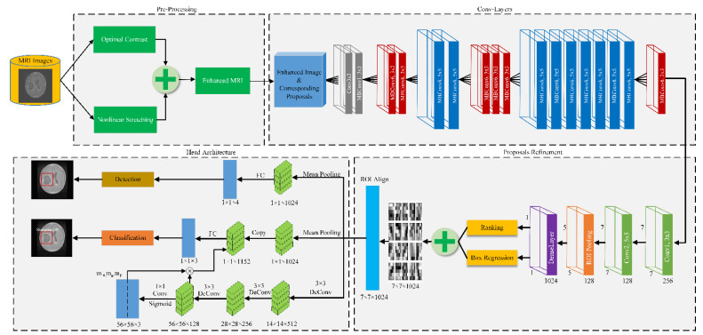
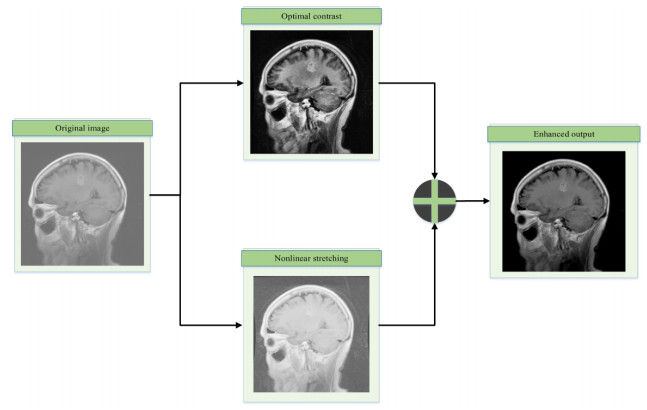
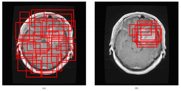
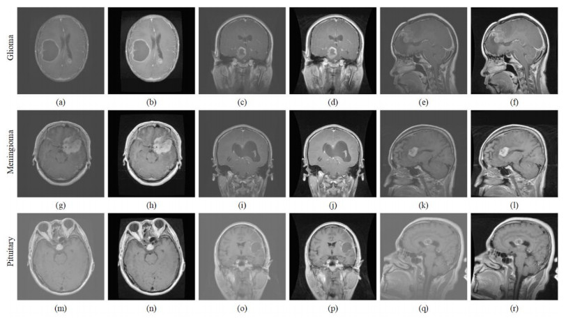
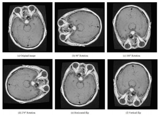
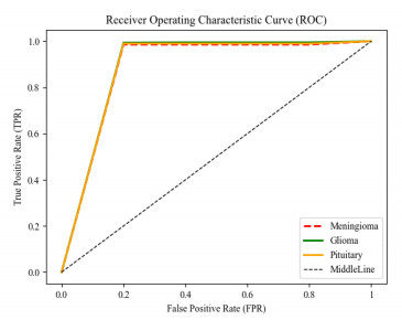
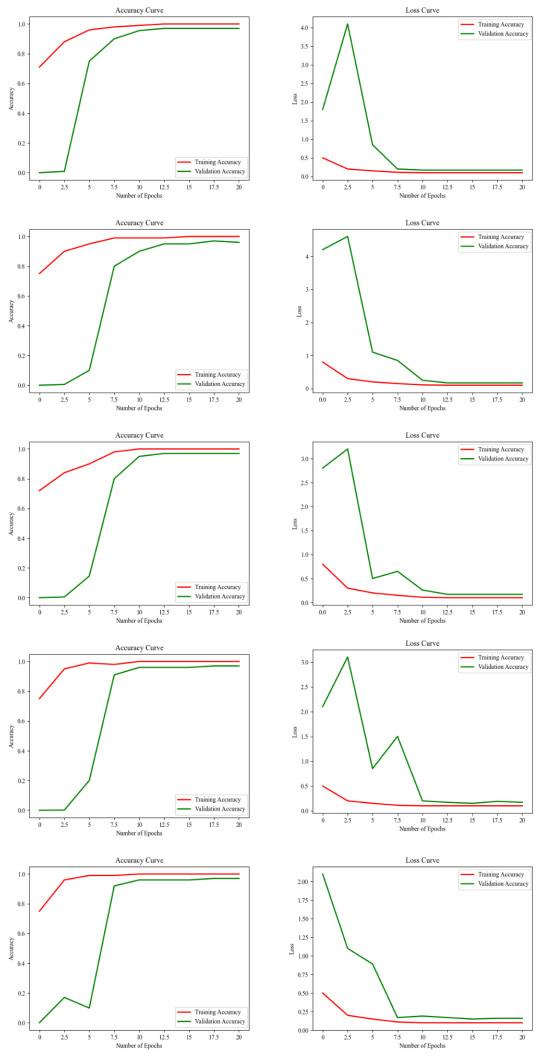
A brain tumor is an abnormal growth of brain cells inside the head, which reduces the patient's survival chance if it is not diagnosed at an earlier stage. Brain tumors vary in size, different in type, irregular in shapes and require distinct therapies for different patients. Manual diagnosis of brain tumors is less efficient, prone to error and time-consuming. Besides, it is a strenuous task, which counts on radiologist experience and proficiency. Therefore, a modern and efficient automated computer-assisted diagnosis (CAD) system is required which may appropriately address the aforementioned problems at high accuracy is presently in need. Aiming to enhance performance and minimise human efforts, in this manuscript, the first brain MRI image is pre-processed to improve its visual quality and increase sample images to avoid over-fitting in the network. Second, the tumor proposals or locations are obtained based on the agglomerative clustering-based method. Third, image proposals and enhanced input image are transferred to backbone architecture for features extraction. Fourth, high-quality image proposals or locations are obtained based on a refinement network, and others are discarded. Next, these refined proposals are aligned to the same size, and finally, transferred to the head network to achieve the desired classification task. The proposed method is a potent tumor grading tool assessed on a publicly available brain tumor dataset. Extensive experiment results show that the proposed method outperformed the existing approaches evaluated on the same dataset and achieved an optimal performance with an overall classification accuracy of 98.04%. Besides, the model yielded the accuracy of 98.17, 98.66, 99.24%, sensitivity (recall) of 96.89, 97.82, 99.24%, and specificity of 98.55, 99.38, 99.25% for Meningioma, Glioma, and Pituitary classes, respectively.
Citation: Yurong Guan, Muhammad Aamir, Ziaur Rahman, Ammara Ali, Waheed Ahmed Abro, Zaheer Ahmed Dayo, Muhammad Shoaib Bhutta, Zhihua Hu. A framework for efficient brain tumor classification using MRI images[J]. Mathematical Biosciences and Engineering, 2021, 18(5): 5790-5815. doi: 10.3934/mbe.2021292
A brain tumor is an abnormal growth of brain cells inside the head, which reduces the patient's survival chance if it is not diagnosed at an earlier stage. Brain tumors vary in size, different in type, irregular in shapes and require distinct therapies for different patients. Manual diagnosis of brain tumors is less efficient, prone to error and time-consuming. Besides, it is a strenuous task, which counts on radiologist experience and proficiency. Therefore, a modern and efficient automated computer-assisted diagnosis (CAD) system is required which may appropriately address the aforementioned problems at high accuracy is presently in need. Aiming to enhance performance and minimise human efforts, in this manuscript, the first brain MRI image is pre-processed to improve its visual quality and increase sample images to avoid over-fitting in the network. Second, the tumor proposals or locations are obtained based on the agglomerative clustering-based method. Third, image proposals and enhanced input image are transferred to backbone architecture for features extraction. Fourth, high-quality image proposals or locations are obtained based on a refinement network, and others are discarded. Next, these refined proposals are aligned to the same size, and finally, transferred to the head network to achieve the desired classification task. The proposed method is a potent tumor grading tool assessed on a publicly available brain tumor dataset. Extensive experiment results show that the proposed method outperformed the existing approaches evaluated on the same dataset and achieved an optimal performance with an overall classification accuracy of 98.04%. Besides, the model yielded the accuracy of 98.17, 98.66, 99.24%, sensitivity (recall) of 96.89, 97.82, 99.24%, and specificity of 98.55, 99.38, 99.25% for Meningioma, Glioma, and Pituitary classes, respectively.

| [1] | T. Zhang, A. H. Sodhro, Z. Luo, N. Zahid, M. W. Nawaz, S. Pirbhulal, et al., A joint deep learning and internet of medical things driven framework for elderly patients, IEEE Access, 8 (2020), 75822-75832. |
| [2] | S. Pirbhulal, W Wu, S. C. Mukhopadhyay, G. Li, Adaptive energy optimization algorithm for internet of medical things, in 2018 12th International Conference on Sensing Technology (ICST), (2018), 269-272. |
| [3] | H. Zhang, H. Zhang, S. Pirbhulal, W. Wu, V. H. Albuquerque, Active balancing mechanism for imbalanced medical data in deep learning-based classification models, ACM Trans. Multimedia Comput., Commun., Appl. (TOMM), 16 (2020), 1-15. |
| [4] |
M. Muzammal, R. Talat, A. H. Sodhro, S. Pirbhulal, A multi-sensor data fusion enabled ensemble approach for medical data from body sensor networks, Inf. Fusion, 53 (2020), 155-164. doi: 10.1016/j.inffus.2019.06.021

|
| [5] | S. Pirbhulal, H. Zhang, W. Wu, S. C. Mukhopadhyay, T. Islam, HRV-based biometric privacy-preserving and security mechanism for wireless body sensor networks, Wearable Sens. Appl. Des. Implementation, (2017), 1-27. |
| [6] | U. K. Acharya, S. Kumar, Genetic algorithm based adaptive histogram equalization (GAAHE) technique for medical image enhancement, Optik, 230 (2021), 166273. |
| [7] |
Y. Zhang, S. Liu, C. Li, J. Wang, Rethinking the dice loss for deep learning lesion segmentation in medical images, J. Shanghai Jiaotong Univ. (Sci.), 26 (2021), 93-102. doi: 10.1007/s12204-021-2264-x
|
| [8] | S. Liang, H. Liu, Y. Gu, X. Guo, H. Li, L. Li, et al., Fast automated detection of COVID-19 from medical images using convolutional neural networks, Commun. Biol., 4 (2021), 1-3. |
| [9] | A. S. Miroshnichenko, V. M. Mikhelev, Classification of medical images of patients with Covid-19 using transfer learning technology of convolutional neural network, in Journal of Physics: Conference Series, 1801 (2021), 012010. |
| [10] | F. Alenezi, K. C. Santosh, Geometric regularized Hopfield neural network for medical image enhancement, Int. J. Biomed. Imaging, 2021 (2021). |
| [11] | R. A. Gougeh, T. Y. Rezaii, A. Farzamnia, Medical image enhancement and deblurring, in Proceedings of the 11th National Technical Seminar on Unmanned System Technology 2019, (2021), 543-554. |
| [12] | Y. Ma, Y. Liu, J. Cheng, Y. Zheng, M. Ghahremani, H. Chen, et al., Cycle structure and illumination constrained GAN for medical image enhancement, in International Conference on Medical Image Computing and Computer-Assisted Intervention, (2020), 667-677. |
| [13] | D. Zhang, G. Huang, Q. Zhang, J. Han, J. Han, Y. Yu, Cross-modality deep feature learning for brain tumor segmentation, Pattern Recognit., 110 (2021), 107562. |
| [14] | N. Heller, F. Isensee, K. H. Maier-Hein, X. Hou, C. Xie, F. Li, et al., The state of the art in kidney and kidney tumor segmentation in contrast-enhanced CT imaging: Results of the kits19 challenge, Med. Image Anal., 67 (2021), 101821. |
| [15] | D. Zhang, B. Chen, J. Chong, S. Li, Weakly-supervised teacher-student network for liver tumor segmentation from non-enhanced images, Med. Image Anal., (2021), 102005. |
| [16] | S. Preethi, P. Aishwarya, An efficient wavelet-based image fusion for brain tumor detection and segmentation over PET and MRI image, Multimedia Tools Appl., (2021), 1-8. |
| [17] | M. Toğaçar, B. Ergen, Z. Cömert, Tumor type detection in brain MR images of the deep model developed using hypercolumn technique, attention modules, and residual blocks, Med. Biol. Eng. Comput., 59 (2021), 57-70. |
| [18] |
B. Kaushal, M. D. Patil, G. K. Birajdar, Fractional wavelet transform based diagnostic system for brain tumor detection in MR imaging, Int. J. Imaging Syst. Technol., 31 (2021), 575-591. doi: 10.1002/ima.22497
|
| [19] | F. J. Díaz-Pernas, M. Martínez-Zarzuela, M. Antón-Rodríguez, D. González-Ortega, A deep learning approach for brain tumor classification and segmentation using a multiscale convolutional neural network, in Healthcare, 9 (2021) 153. |
| [20] | A. R. Khan, S. Khan, M. Harouni, R. Abbasi, S. Iqbal, Z. Mehmood, Brain tumor segmentation using K‐means clustering and deep learning with synthetic data augmentation for classification, Microsc. Res. Tech., 2021. |
| [21] | C. L. Maire, M. M. Fuh, K. Kaulich, K. D. Fita, I. Stevic, D. H. Heiland, et al., Genome-wide methylation profiling of glioblastoma cell-derived extracellular vesicle DNA allows tumor classification, Neuro-oncology, 2021. |
| [22] | G. Garg, R. Garg, Brain tumor detection and classification based on hybrid ensemble classifier, preprint, arXiv: 2101.00216. |
| [23] | K. Kaplan, Y. Kaya, M. Kuncan, H. M. Ertunç, Brain tumor classification using modified local binary patterns (LBP) feature extraction methods, Med. Hypotheses, 139 (2020), 109696. |
| [24] |
J. Amin, M. Sharif, N. Gul, M. Yasmin, S. A. Shad, Brain tumor classification based on DWT fusion of MRI sequences using convolutional neural network, Pattern Recognit. Lett., 129 (2020), 115-122. doi: 10.1016/j.patrec.2019.11.016
|
| [25] | N. Ghassemi, A. Shoeibi, M. Rouhani, Deep neural network with generative adversarial networks pre-training for brain tumor classification based on MR images, Biomed. Signal Process. Control, 57 (2020), 101678. |
| [26] | A. M. Alhassan, W. M. Zainon, Brain tumor classification in magnetic resonance image using hard swish-based RELU activation function-convolutional neural network, Neural Comput. Appl., (2021), 1-3. |
| [27] |
M. Agarwal, G. Rani, V. S. Dhaka, Optimized contrast enhancement for tumor detection, Int. J. Imaging Syst. Technol., 30 (2020), 687-703. doi: 10.1002/ima.22408
|
| [28] | B. S. Rao, Dynamic histogram equalization for contrast enhancement for digital images, Appl. Soft Comput., 89 (2020), 106114. |
| [29] |
B. Subramani, M. Veluchamy, A fast and effective method for enhancement of contrast resolution properties in medical images, Multimedia Tools Appl., 79 (2020), 7837-7855. doi: 10.1007/s11042-018-6434-2
|
| [30] | Z. Ullah, M. U. Farooq, S. H. Lee, D. An, A hybrid image enhancement based brain MRI images classification technique, Med. Hypotheses, 143 (2020), 109922. |
| [31] | U. K. Acharya, S. Kumar, Particle swarm optimized texture based histogram equalization (PSOTHE) for MRI brain image enhancement, Optik, 224 (2020), 165760. |
| [32] | J. Cheng, W. Huang, S. Cao, R. Yang, W. Yang, Z. Yun, et al., Enhanced performance of brain tumor classification via tumor region augmentation and partition, PloS One, 10 (2015), e0140381. |
| [33] | M. R. Ismael, I. Abdel-Qader, Brain tumor classification via statistical features and back-propagation neural network, in 2018 IEEE International Conference on Electro/Information Technology (EIT), IEEE, (2018), 252-257. |
| [34] | B. Tahir, S. Iqbal, M. Usman Ghani Khan, T. Saba T, Z. Mehmood, A. Anjum, et al., Feature enhancement framework for brain tumor segmentation and classification, Microscopy Res. Tech., 82 (2019), 803-811. |
| [35] | J. S. Paul, A. J. Plassard, B. A. Landman, D. Fabbri, Deep learning for brain tumor classification, in Medical Imaging 2017: Biomedical Applications in Molecular, Structural, and Functional Imaging, 10137 (2017), 1013710. |
| [36] | P. Afshar, A. Mohammadi, K. N. Plataniotis, Brain tumor type classification via capsule networks, in 2018 25th IEEE International Conference on Image Processing (ICIP), IEEE, (2018), 3129-3133, |
| [37] | P. Afshar, K. N. Plataniotis, A. Mohammadi, Capsule networks for brain tumor classification based on MRI images and coarse tumor boundaries, in ICASSP 2019-2019 IEEE International Conference on Acoustics, Speech and Signal Processing (ICASSP), IEEE, (2019), 1368-1372. |
| [38] | Y. Zhou, Z. Li, H. Zhu, C. Chen, M. Gao, K. Xu, et al., Holistic brain tumor screening and classification based on densenet and recurrent neural network, in International MICCAI Brain lesion Workshop, Springer, Cham, (2018), 208-217. |
| [39] | A. Pashaei, H. Sajedi, N. Jazayeri, Brain tumor classification via convolutional neural network and extreme learning machines, in 2018 8th International Conference on Computer and Knowledge Engineering (ICCKE), IEEE, (2018), 314-319. |
| [40] | N. Abiwinanda, M. Hanif, S. T. Hesaputra, A. Handayani, T. R. Mengko, Brain tumor classification using convolutional neural network, in World Congress on Medical Physics and Biomedical Engineering 2018, Springer, Singapore, (2019), 183-189. |
| [41] | J. Guo, W. Qiu, X. Li, X. Zhao, N. Guo, Q. Li, Predicting alzheimer's disease by hierarchical graph convolution from positron emission tomography imaging, in 2019 IEEE International Conference on Big Data (Big Data), IEEE, (2019), 5359-5363. |
| [42] |
W. Ayadi, W. Elhamzi, I. Charfi, M. Atri, Deep CNN for brain tumor classification, Neural Process. Lett., 53 (2021), 671-700. doi: 10.1007/s11063-020-10398-2
|
| [43] | S. Deepak, P. M. Ameer, Brain tumor classification using deep CNN features via transfer learning, Comput. Biol. Med., 111 (2019), 103345. |
| [44] |
P. F. Felzenszwalb, D. P. Huttenlocher, Efficient graph-based image segmentation, Int. J. Comput. Vision, 59 (2004), 167-181. doi: 10.1023/B:VISI.0000022288.19776.77
|
| [45] | M. Aamir, Y. F. Pu, Z. Rahman, W. A. Abro, H. Naeem, F. Ullah, et al., A hybrid proposed framework for object detection and classification, J. Inf. Process. Syst., 14 (2018). |
| [46] | M. Aamir, Y. F. Pu, W. A. Abro, H. Naeem, Z. Rahman, A hybrid approach for object proposal generation, in International Conference on Sensing and Imaging, Springer, Cham, (2017), 251-259. |
| [47] | M. Tan, Q. Le, Efficientnet: Rethinking model scaling for convolutional neural networks, in International Conference on Machine Learning, PMLR, (2019), 6105-6114. |
| [48] | Y. Guan, M. Aamir, Z. Hu, W. A. Abro, Z. Rahman, Z. A. Dayo, et al., A region-based efficient network for accurate object detection, Trait. du Signal, 38 (2021). |
| [49] | M. Sandler, A. Howard, M. Zhu M, A. Zhmoginov, L. C. Chen, Mobilenetv2: Inverted residuals and linear bottlenecks, in Proceedings of the IEEE Conference on Computer Vision and Pattern Recognition, (2018), 4510-4520. |
| [50] | R. Girshick, Fast r-cnn, in Proceedings of the IEEE International Conference on Computer Vision, (2015), 1440-1448. |
| [51] | T. Sadad, A. Rehman, A. Munir, T. Saba, U. Tariq, N. Ayesha, et al., Brain tumor detection and multi‐classification using advanced deep learning techniques, Microscopy Res. Tech., 84 (2021), 1296-1308. |
| [52] |
A. Rehman, S. Naz, M. I. Razzak, F. Akram, M. Imran, A deep learning-based framework for automatic brain tumors classification using transfer learning, Circuits, Syst. Signal Process., 39 (2020), 757-775. doi: 10.1007/s00034-019-01246-3
|
| [53] |
Z. Rahman, Y. F. Pu, M. Aamir, S. Wali, Structure revealing of low-light images using wavelet transform based on fractional-order denoising and multiscale decomposition, Visual Comput., 37 (2021), 865-880. doi: 10.1007/s00371-020-01838-0
|
| [54] | M. Aamir, Z. Rahman, Y. F. Pu, W. A. Abro, K. Gulzar, Satellite image enhancement using wavelet-domain based on singular value decomposition, Int. J. Adv. Comput. Sci. Appl. (IJACSA), 2019. |
| [55] | M. Aamir, Z. Rehman, Y. F. Pu, A. Ahmed, W. A. Abro, Image enhancement in varying light conditions based on wavelet transform, in 2019 16th International Computer Conference on Wavelet Active Media Technology and Information Processing, (2019), 317-322. |
| [56] | M. Aamir, Y. F. Pu, Z. Rahman, M. Tahir, H. Naeem, Q. Dai, A framework for automatic building detection from low-contrast satellite images, Symmetry, 11 (2019), 3. |
Figures(9) / Tables(7)

Yurong Guan, Muhammad Aamir, Ziaur Rahman, Ammara Ali, Waheed Ahmed Abro, Zaheer Ahmed Dayo, Muhammad Shoaib Bhutta, Zhihua Hu. A framework for efficient brain tumor classification using MRI images[J]. Mathematical Biosciences and Engineering, 2021, 18(5): 5790-5815. doi: 10.3934/mbe.2021292


 DownLoad: