Cloud manufacturing (CM) establishes a collaborative manufacturing services chain among dispersed producers, which enables the efficient satisfaction of personalized manufacturing requirements. To further strengthen this effect, the manufacturing service composition and optimal selection (SCOS) in CM, as a NP-hard combinatorial problem, is a crucial issue. Quality of service (QoS) attributes of manufacturing services, as the basic criterion of functions and capabilities, are decisive criterions of SCOS. However, most traditional QoS attributes of CM ignore the dynamic equilibrium of manufacturing services and only rely on initial static characterizations such as reliability and availability. In a high uncertainty and dynamicity environment, a major concern is the equilibrium of manufacturing services for recovering their functions after dysfunctional damage. Therefore, this paper proposes a hybrid resilience-aware global optimization (HRGO) approach to address the SCOS problem in CM. This approach helps manufacturing demanders to acquire efficient, resilient, and satisfying manufacturing services. First, the problem description and resilience measurement method on resilience-aware SCOS is modeled. Then, a services filter strategy, based on the fuzzy similarity degree, is introduced to filter redundant and unqualified candidate services. Finally, a modified non-dominated sorting genetic algorithm (MNSGA-III) is proposed, based on diversity judgment and dualtrack parallelism, to address combination optimization processing in SCOS. A series of experiments were conducted, the results show the proposed method is more preferable in optimal services searching and more efficient in scalability.
Citation: Hao Song, Xiaonong Lu, Xu Zhang, Xiaoan Tang, Qiang Zhang. A HRGO approach for resilience enhancement service composition and optimal selection in cloud manufacturing[J]. Mathematical Biosciences and Engineering, 2020, 17(6): 6838-6872. doi: 10.3934/mbe.2020355
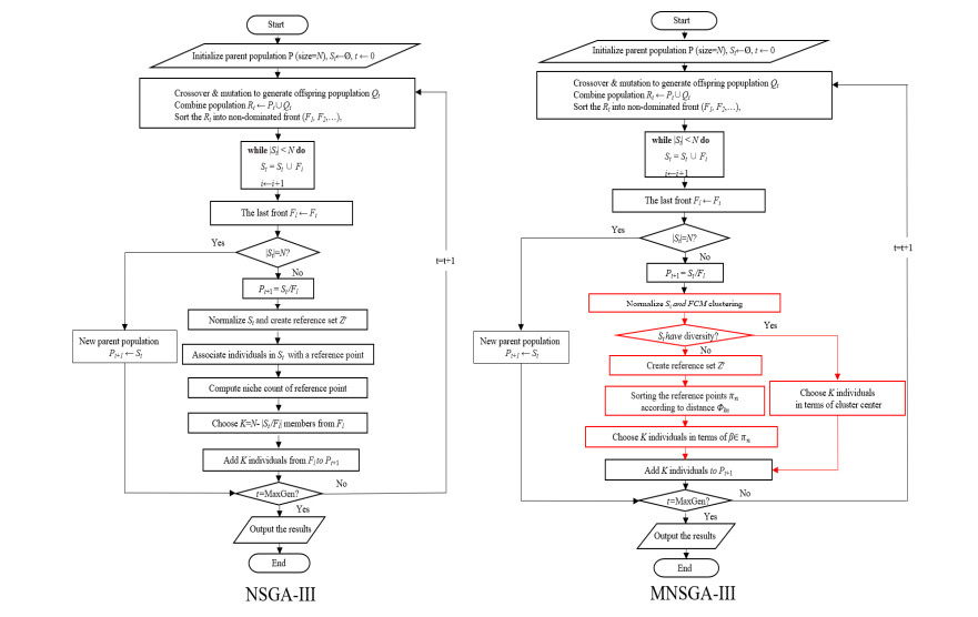
Cloud manufacturing (CM) establishes a collaborative manufacturing services chain among dispersed producers, which enables the efficient satisfaction of personalized manufacturing requirements. To further strengthen this effect, the manufacturing service composition and optimal selection (SCOS) in CM, as a NP-hard combinatorial problem, is a crucial issue. Quality of service (QoS) attributes of manufacturing services, as the basic criterion of functions and capabilities, are decisive criterions of SCOS. However, most traditional QoS attributes of CM ignore the dynamic equilibrium of manufacturing services and only rely on initial static characterizations such as reliability and availability. In a high uncertainty and dynamicity environment, a major concern is the equilibrium of manufacturing services for recovering their functions after dysfunctional damage. Therefore, this paper proposes a hybrid resilience-aware global optimization (HRGO) approach to address the SCOS problem in CM. This approach helps manufacturing demanders to acquire efficient, resilient, and satisfying manufacturing services. First, the problem description and resilience measurement method on resilience-aware SCOS is modeled. Then, a services filter strategy, based on the fuzzy similarity degree, is introduced to filter redundant and unqualified candidate services. Finally, a modified non-dominated sorting genetic algorithm (MNSGA-III) is proposed, based on diversity judgment and dualtrack parallelism, to address combination optimization processing in SCOS. A series of experiments were conducted, the results show the proposed method is more preferable in optimal services searching and more efficient in scalability.

| [1] | S. Mejjaouli, R. F. Babiceanu, T. Borangiu, D. Trentesaux, Service Orientation in Holonic and Multi-Agent Manufacturing and Robotics, Springer International Publishing, (2014), 31-46. |
| [2] | R. F. Babiceanu, R. Seker in T. Borangiu, A. Thomas, Service Orientation in Holonic and Multi-Agent Manufacturing, Springer International Publishing, (2015), 165-173. |
| [3] |
Y. Wang, A Formal Model of QoS-Aware Web Service Orchestration Engine, IEEE Trans. Network Serv. Manage., 13 (2016), 113-125. doi: 10.1109/TNSM.2015.2507166

|
| [4] | J. Tapolcai, P. Cholda, T. Cinkler, K. Wajda, A. Jajszczyk, A. Autenrieth, et al., Quality of resilience (QoR): NOBEL approach to the multi-service resilience characterization, 2nd International Conference on Broadband Networks, 2005. Available from: https://ieeexplore.ieee.org/abstract/document/1589762. |
| [5] |
S. K. Pradhan, S. Routroy, Development of supply chain risk mitigation strategy: a case study, Int. J. Procurement Manage., 7 (2014), 359-375. doi: 10.1504/IJPM.2014.063166
|
| [6] |
S. Huang, S. Zeng, Y. Fan, G. Q. Huang, Optimal service selection and composition for service-oriented manufacturing network, Int. J. Comput. Integr. Manuf., 24 (2011), 416-430. doi: 10.1080/0951192X.2010.511657
|
| [7] |
Q. Zhang, X. Lu, Z. Peng, M. Ren, Perspective: a review of lifecycle management research on complex products in smart-connected environments, Int. J. Prod. Res., 57 (2019), 6758-6779. doi: 10.1080/00207543.2019.1587186
|
| [8] |
J. Yi, C. Lu, G. Li, A literature review on latest developments of Harmony Search and its applications to intelligent manufacturing, Math. Biosci. Eng., 16 (2019), 2086-2117. doi: 10.3934/mbe.2019102
|
| [9] |
Y. Suresh, T. Kalaivani, J. Senthilkumar, V. Mohanraj, BF2 VHDR based dynamic routing with hydrodynamics for QoS development in WSN, Math. Biosci. Eng., 17 (2020), 930-947. doi: 10.3934/mbe.2020050
|
| [10] |
M. S. Rahman, I. Khalil, A. Alabdulatif, X. Yi, Privacy preserving service selection using fully homomorphic encryption scheme on untrusted cloud service platform, Knowl. Based Syst., 180 (2019), 104-115. doi: 10.1016/j.knosys.2019.05.022
|
| [11] |
Y. Cao, S. Wang, L. Kang, Y. Gao, A TQCS-based service selection and scheduling strategy in cloud manufacturing, Int. J. Adv. Manuf. Technol., 82 (2016), 235-251. doi: 10.1007/s00170-015-7350-5
|
| [12] |
B. Huang, C. Li, F. Tao, A chaos control optimal algorithm for QoS-based service composition selection in cloud manufacturing system, Enterp. Inf. Syst., 8 (2014), 445-463. doi: 10.1080/17517575.2013.792396
|
| [13] |
Y. K. Lin, C. S. Chong, Fast GA-based project scheduling for computing resources allocation in a cloud manufacturing system, J. Intell. Manuf., 28 (2017), 1189-1201. doi: 10.1007/s10845-015-1074-0
|
| [14] |
Y. Laili, F. Tao, L, Zhang, B. R. Sarker, A study of optimal allocation of computing resources in cloud manufacturing systems, Int. J. Adv. Manuf. Technol., 63 (2012), 671-690. doi: 10.1007/s00170-012-3939-0
|
| [15] |
W. Liu, B. Liu, D. Sun, Y. Li, G. Ma, Study on multi-task oriented services composition and optimisation with the 'Multi-Composition for Each Task' pattern in cloud manufacturing systems, Int. J. Comput. Integr. Manuf., 26 (2013), 786-805. doi: 10.1080/0951192X.2013.766939
|
| [16] | M. Alrifai, T. Risse, A Hybrid Approach for Efficient Web Service Composition with End-to-End QoS Constraints, ACM Trans. Web, 2 (2012), 7. |
| [17] | W. Xu, S. Tian, Q. Liu, Y. Xie, Z. Zhou, D. T, Pham, An improved discrete bees algorithm for correlation-aware service aggregation optimization in cloud manufacturing, Int. J. Adv. Manuf. Technol., 84 (2016), 17-28. |
| [18] |
J. Zhou, X. Yao, Multi-population parallel self-adaptive differential artificial bee colony algorithm with application in large-scale service composition for cloud manufacturing, Appl. Soft Comput., 56 (2017), 379-397. doi: 10.1016/j.asoc.2017.03.017
|
| [19] |
F. Xiang, Y. Hu, Y. Yu, H. Wu, QoS and energy consumption aware service composition and optimal-selection based on Pareto group leader algorithm in cloud manufacturing system, Cent. Eur. J. Oper. Res., 22 (2014), 663-685. doi: 10.1007/s10100-013-0293-8
|
| [20] |
H. Jin, X. Yao, Y. Chen, Correlation-aware QoS modeling and manufacturing cloud service composition, J. Intell. Manuf., 28 (2017), 1947-1960. doi: 10.1007/s10845-015-1080-2
|
| [21] | W. Zhang, Y. Yang, S. Zhang, D. Yu, Y. Xu, A New Manufacturing Service Selection and Composition Method Using Improved Flower Pollination Algorithm, Math. Probl. Eng., 2016 (2016), 1-12. |
| [22] |
J. Zhou, X. Yao, DE-caABC: differential evolution enhanced context-aware artificial bee colony algorithm for service composition and optimal selection in cloud manufacturing, Int. J. Adv. Manuf. Technol., 90 (2017), 1085-1103. doi: 10.1007/s00170-016-9455-x
|
| [23] |
J. Lartigau, X. Xu, L. Nie, D. Zhan, Cloud manufacturing service composition based on QoS with geo-perspective transportation using an improved Artificial Bee Colony optimisation algorithm, Int. J. Prod. Res., 53 (2015), 4380-4404. doi: 10.1080/00207543.2015.1005765
|
| [24] |
J. Zhou, X. Yao, Hybrid teaching-learning-based optimization of correlation-aware service composition in cloud manufacturing, Int. J. Adv. Manuf. Technol., 91 (2017), 3515-3533. doi: 10.1007/s00170-017-0008-8
|
| [25] |
Y. Cao, S. Wang, L. Kang, C. Li, L. Guo, Study on machining service modes and resource selection strategies in cloud manufacturing, Int. J. Adv. Manuf. Technol., 81 (2015), 597-613. doi: 10.1007/s00170-015-7222-z
|
| [26] |
F. Seghir, A. Khababa, A hybrid approach using genetic and fruit fly optimization algorithms for QoS-aware cloud service composition, J. Intell. Manuf., 29 (2018), 1773-1792. doi: 10.1007/s10845-016-1215-0
|
| [27] |
B. Xu, Z. Sun, A fuzzy operator based bat algorithm for cloud service composition, Int. J. Wireless Mobile Comput., 11 (2016), 42-46. doi: 10.1504/IJWMC.2016.079471
|
| [28] |
J. Zhou, X. Yao, Multi-objective hybrid artificial bee colony algorithm enhanced with Lévy flight and self-adaption for cloud manufacturing service composition, Appl. Intell., 47 (2017), 721-742. doi: 10.1007/s10489-017-0927-y
|
| [29] |
B. Liu, Z. Zhang, QoS-aware service composition for cloud manufacturing based on the optimal construction of synergistic elementary service groups, Int. J. Adv. Manuf. Technol., 88 (2017), 2757-2771. doi: 10.1007/s00170-016-8992-7
|
| [30] |
X. Gu, X. Jin, J. Ni, Y. Koren, Manufacturing System Design for Resilience, Procedia CIRP, 36 (2015), 135-140. doi: 10.1016/j.procir.2015.02.075
|
| [31] | W. J. Zhang, C. A, van Luttervelt, Toward a resilient manufacturing system, CIRP Ann., 60 (2011), 469-472. |
| [32] | L. Zhang, H. Guo, F. Tao, Y. L. Luo, Flexible management of resource service composition in cloud manufacturing, 2010 IEEE International Conference on Industrial Engineering and Engineering Management, 2010. Available from: https://ieeexplore.ieee.org/abstract/document/5674175/. |
| [33] | F. Tao, L. Zhang, Y. Liu, Y. Cheng, L. Wang, X. Xu, Manufacturing Service Management in Cloud Manufacturing: Overview and Future Research Directions, J. Manuf. Sci. Eng. Trans., 137 (2015). |
| [34] | S. S. Shah, R. F. Babiceanu, Resilience Modeling and Analysis of Interdependent Infrastructure Systems, Syst. Inf. Eng. Des. Symp., 2015 (2015), 154-158. |
| [35] |
R. Francis, B. Bekera, A metric and frameworks for resilience analysis of engineered and infrastructure systems, Reliab. Eng. Syst. Saf., 121 (2014), 90-103. doi: 10.1016/j.ress.2013.07.004
|
| [36] |
M. Ouyang, Review on modeling and simulation of interdependent critical infrastructure systems, Reliab. Eng. Syst. Saf., 121 (2014), 43-60. doi: 10.1016/j.ress.2013.06.040
|
| [37] | P. É rdi, Complexity Explained, Springer Science & Business Media, (2007). |
| [38] |
W. Y. Zhang, S. Zhang, M. Cai, J. X. Huang, A new manufacturing resource allocation method for supply chain optimization using extended genetic algorithm, Int. J. Adv. Manuf. Technol., 53 (2011), 1247-1260. doi: 10.1007/s00170-010-2900-3
|
| [39] |
M. R. Namjoo, A. Keramati, Analysing Causal dependencies of composite service resilience in cloud manufacturing using resource-based theory and DEMATEL method, Int. J. Comput. Integr. Manuf., 31 (2018), 942-960. doi: 10.1080/0951192X.2018.1493231
|
| [40] |
T. Y. Tseng, C. M. Klein, New algorithm for the ranking procedure in fuzzy decision-making, IEEE Trans. Syst. Man Cyber., 19 (1989), 1289-1296. doi: 10.1109/21.44050
|
| [41] |
K. Sindhya, K. Miettinen, K. Deb, A Hybrid Framework for Evolutionary Multi-Objective Optimization, IEEE Trans. Evol. Comput., 17 (2013), 495-511. doi: 10.1109/TEVC.2012.2204403
|
| [42] |
Y. Hua, Y. Jin, K. Hao, A Clustering-Based Adaptive Evolutionary Algorithm for Multi-objective Optimization with Irregular Pareto Fronts, IEEE Trans. Cyber., 49 (2019), 2758-2770. doi: 10.1109/TCYB.2018.2834466
|
| [43] | K. Deb, H. Jain, An Evolutionary Many-Objective Optimization Algorithm Using Reference-Point-Based Nondominated Sorting Approach, Part I: Solving Problems With Box Constraints, IEEE Trans. Evol. Comput., 18 (2014), 577-601. |
| [44] | Hui. Li, Q. F. Zhang, Multiobjective Optimization Problems with Complicated Pareto Sets, MOEA/D and NSGA-II, IEEE Trans. Evol. Comput., 13 (2009), 284-302. |
| [45] | K. Deb, R. B. Agrawal, Simulated Binary Crossover for Continuous Search Space, Complex Syst., 9 (1995), 115-148. |
| [46] |
P. M. Pardalos, I. Steponavičė, A. Zilinskas, Pareto set approximation by the method of adjustable weights and successive lexicographic goal programming, Optim. Lett., 6 (2012), 665-678. doi: 10.1007/s11590-011-0291-5
|
| [47] |
K. Deb, A. Pratap, S. Agarwal, T. Meyarivan, A fast and elitist multi-objective genetic algorithm: NSGA-II, IEEE Trans. Evol. Comput., 6 (2002), 182-197. doi: 10.1109/4235.996017
|
| [48] |
S. Guo, B. Du, Z. Peng, X. Huang, Y. Li, Manufacturing resource combinatorial optimization for large complex equipment in group manufacturing: A cluster-based genetic algorithm, Mechatronics, 31 (2015), 101-115. doi: 10.1016/j.mechatronics.2015.03.005
|
| [49] |
H. Zheng, Y. Feng, J. Tan, A fuzzy QoS-aware resource service selection considering design preference in cloud manufacturing system, Int. J. Adv. Manuf. Technol., 84 (2016), 371-379. doi: 10.1007/s00170-016-8417-7
|
| [50] |
Q. F. Zhang, H. Li, MOEA/D: A Multi-objective Evolutionary Algorithm Based on Decomposition, IEEE Trans. Evol. Comput., 11 (2007), 712-731. doi: 10.1109/TEVC.2007.892759
|
| [51] |
M. E. Khanouche, F. Attal, Y. Amirat, A. Chibani, M. Kerkar, Clustering-based and QoS-aware services composition algorithm for ambient intelligence, Infor. Sci., 482 (2019), 419-439. doi: 10.1016/j.ins.2019.01.015
|
| [52] |
H. Ishibuchi, N. Akedo, Y. Nojima, Behavior of Multiobjective Evolutionary Algorithms on Many-Objective Knapsack Problems, IEEE Trans. Evol. Comput., 19 (2015), 264-283. doi: 10.1109/TEVC.2014.2315442
|
| [53] | M. R. Namjoo, A. Keramati, S. A. Torabi, F. Jolai, Quantifying the Resilience of Cloud-Based Manufacturing Composite Services, Int. J. Cloud Appl. Comput., 8 (2018), 88-117. |
Figures(12) / Tables(12)

Hao Song, Xiaonong Lu, Xu Zhang, Xiaoan Tang, Qiang Zhang. A HRGO approach for resilience enhancement service composition and optimal selection in cloud manufacturing[J]. Mathematical Biosciences and Engineering, 2020, 17(6): 6838-6872. doi: 10.3934/mbe.2020355


 DownLoad: