Research article Special Issues

Reliable data transmission in wireless sensor networks with data decomposition and ensemble recovery

  • Wireless sensor networks (WSNs) are usually used to helps many basic scientific works to gather and observe environmental data, whose completeness and accuracy are the key to ensuring the success of scientific works. However, due to a lot of noise, collision and unreliable data link, data loss and damage in WSNs are rather common. Although some existing works, e.g. interpolation methods or prediction methods, can recover original data to some extent, they maybe provide an unsatisfactory accuracy when the missing data becomes large. To address this problem, this paper proposes a new reliable data transmission scheme in WSNs by using data decomposition and ensemble recovery mechanism. Firstly, the original data are collected by sensor nodes and then are expanded and split into multiple data shares by using multi-ary Vandermonde matrix. Subsequently, these data shares are transmitted respectively to source node via the sensor networks, which is made up of a large number of sensor nodes. Since each share contains data redundancy, the source node can reconstruct the original data even if some data shares are damaged or lost during delivery. Finally, extensive simulation experiments show that the proposed scheme outperforms significantly existing solutions in terms of recovery accuracy and robustness.

    Citation: Fengyong Li, Gang Zhou, Jingsheng Lei. Reliable data transmission in wireless sensor networks with data decomposition and ensemble recovery[J]. Mathematical Biosciences and Engineering, 2019, 16(5): 4526-4545. doi: 10.3934/mbe.2019226

    Related Papers:

    [1] Noman Zahid, Ali Hassan Sodhro, Usman Rauf Kamboh, Ahmed Alkhayyat, Lei Wang . AI-driven adaptive reliable and sustainable approach for internet of things enabled healthcare system. Mathematical Biosciences and Engineering, 2022, 19(4): 3953-3971. doi: 10.3934/mbe.2022182
    [2] Hao Yuan, Qiang Chen, Hongbing Li, Die Zeng, Tianwen Wu, Yuning Wang, Wei Zhang . Improved beluga whale optimization algorithm based cluster routing in wireless sensor networks. Mathematical Biosciences and Engineering, 2024, 21(3): 4587-4625. doi: 10.3934/mbe.2024202
    [3] Tingting Yang, Yi He . Design of intelligent robots for tourism management service based on green computing. Mathematical Biosciences and Engineering, 2023, 20(3): 4798-4815. doi: 10.3934/mbe.2023222
    [4] Angel Martin-del Rey . A novel model for malware propagation on wireless sensor networks. Mathematical Biosciences and Engineering, 2024, 21(3): 3967-3998. doi: 10.3934/mbe.2024176
    [5] Naila Naz, Muazzam A Khan, Suliman A. Alsuhibany, Muhammad Diyan, Zhiyuan Tan, Muhammad Almas Khan, Jawad Ahmad . Ensemble learning-based IDS for sensors telemetry data in IoT networks. Mathematical Biosciences and Engineering, 2022, 19(10): 10550-10580. doi: 10.3934/mbe.2022493
    [6] Haitao Huang, Min Tian, Jie Zhou, Xiang Liu . Reliable task allocation for soil moisture wireless sensor networks using differential evolution adaptive elite butterfly optimization algorithm. Mathematical Biosciences and Engineering, 2023, 20(8): 14675-14698. doi: 10.3934/mbe.2023656
    [7] B. Kiruthika, Shyamala Bharathi P . Intelligent dynamic trust secure attacker detection routing for WSN-IoT networks. Mathematical Biosciences and Engineering, 2023, 20(2): 4243-4257. doi: 10.3934/mbe.2023198
    [8] Peng-Yeng Yin, Chih-Chun Tsai, Rong-Fuh Day, Ching-Ying Tung, Bir Bhanu . Ensemble learning of model hyperparameters and spatiotemporal data for calibration of low-cost PM2.5 sensors. Mathematical Biosciences and Engineering, 2019, 16(6): 6858-6873. doi: 10.3934/mbe.2019343
    [9] Faten S. Alamri, Khalid Haseeb, Tanzila Saba, Jaime Lloret, Jose M. Jimenez . Multimedia IoT-surveillance optimization model using mobile-edge authentic computing. Mathematical Biosciences and Engineering, 2023, 20(11): 19174-19190. doi: 10.3934/mbe.2023847
    [10] Huanhai Yang, Shue Liu . A prediction model of aquaculture water quality based on multiscale decomposition. Mathematical Biosciences and Engineering, 2021, 18(6): 7561-7579. doi: 10.3934/mbe.2021374
  • Wireless sensor networks (WSNs) are usually used to helps many basic scientific works to gather and observe environmental data, whose completeness and accuracy are the key to ensuring the success of scientific works. However, due to a lot of noise, collision and unreliable data link, data loss and damage in WSNs are rather common. Although some existing works, e.g. interpolation methods or prediction methods, can recover original data to some extent, they maybe provide an unsatisfactory accuracy when the missing data becomes large. To address this problem, this paper proposes a new reliable data transmission scheme in WSNs by using data decomposition and ensemble recovery mechanism. Firstly, the original data are collected by sensor nodes and then are expanded and split into multiple data shares by using multi-ary Vandermonde matrix. Subsequently, these data shares are transmitted respectively to source node via the sensor networks, which is made up of a large number of sensor nodes. Since each share contains data redundancy, the source node can reconstruct the original data even if some data shares are damaged or lost during delivery. Finally, extensive simulation experiments show that the proposed scheme outperforms significantly existing solutions in terms of recovery accuracy and robustness.


    Wireless Sensor Networks (WSNs) is a multi-hop wireless network that is formed by self-organizing the sensor nodes of large-scale deployment. By WSNs, the data information of the perceived object in the monitoring area is collected and transmitted by a coordinated manner. Since WSNs has more advantages, e.g. strong environment adaptiveness, portable and energy efficient, they are widely used to collect information from the physical world and produce large-scale sensor data sets. Obviously, the completeness and accuracy of these awareness data sets significantly affect the reliability of scientific results. If these data are lost or jumping during transmission, it will inevitably lead to the unreliable or error results. Therefore, the completeness and accuracy for scientific data are so important in decision-making. Nevertheless, in actual data collection scenario, data loss is so common. The reasons can be summarized as follows: (1) wireless channel instability and noise interference, (2) mutual interference between channels caused by tree or clustered topology, (3) congestion caused by data bursts in high-density deployments or emergencies, (4) unexpected failure due to node damage or battery problem. The mentioned cases maybe cause serious errors in receiving end and finally lead to invalidation of some scientific research and engineering calculations.

    Although the importance of missing data in wireless sensor networks is very prominent, the research on this problem is still relatively rare. Some researchers have tried to reconstruct the missing data by using some typical interpolation algorithms [1], which always appear in the field of database [2], multimedia [2], and signal processing [3]. For example, as a classical local interpolation method, k-Nearest-Neighbor (kNN) [4] is usually used to estimate the missing data according to the nearest k neighbors around the missing data position. This scheme can achieve a good estimation performance due to high correlation between adjacent data, and is thus used in low-fidelity estimation cases. Delaunay Triangulation (DT) [5] is another typical global interpolation method. This method considers each collected data as vertices, which are connected into triangles according to the process of gradually reducing the global error, and the missing values are finally inserted into the data set. Multi-channel Singular Spectrum Analysis (MSSA) [6] is a nonparametric adaptive method, which belongs to the category of principal component analysis. This method uses embedded self-covariance matrix to insert missing values. Compressive Sensing (CS) method [7,8] was proposed in 2006, which is an advanced data recovery algorithm. If the data set is sparse, CS method can efficiently estimate the whole data set by using very little known data. Therefore, this method has attracted much research interest. On the basis of CS scheme, Kong et al. proposed an improved algorithm [9], named by Environmental Space Time Improved Compressive Sensing (ESTI-CS), which embeds customized features into the baseline CS to deal with the specific data loss patterns and then uses a multi-attribute assistant (MAA) component to perform data reconstruction. Chen et al. proposed a novel data reconstruction scheme via temporal stability guided matrix completion [10]. They formulate the data reconstruction problem as a matrix completion with structural noise and further reduce the reconstruction error by introducing a constraint about short-term stability to the matrix completion problem.

    Although the existing schemes can work for the data recovery and reconstruction, they can not completely solve the data loss in the wireless sensor network due to the following reasons:

    ● The data loss mechanism in wireless sensor networks has some special characteristics, which often do not meet the assumptions of classical interpolation algorithms.

    ● Existing schemes always reconstruct missing data by interpolation or prediction, which makes that some predicted data are not exactly consistent with the original data. Therefore, they cannot be applied in some cases that needs high data accuracy.

    ● Existing schemes can recover original data only when the missing data is small. In other words, they maybe provide an unsatisfactory accuracy when the missing data becomes large.

    Overall, existing methods always provide the estimated value for the loss data. This mechanism is usually efficient to small-scale insensitive environmental data, but for large-scale and high accuracy data, it may not work well anymore. Facing the aforementioned problems, this paper designs a data decomposition and ensemble recovery mechanism, and tries to fundamentally solve the data loss and jumping in the data transmission for wireless sensor networks. Comparing with the previous works, we make the following novel contributions.

    ● We propose a reliable data transmission scheme by designing data decomposition and ensemble recovery mechanism. We claim that proposed scheme can solve the data loss problem in WSNs, and guarantee the correctness of original data even if some data are lost or damaged in delivery.

    ● We use matrix decomposition to design data expansion mechanism, and then split the original data into multiple data shares, which are transmitted through multiple sensor nodes. Since each data share contains some data redundancy, the loss of part of the shares does not affect the recovery of original data.

    ● Ensemble recovery mechanism is designed to reconstruct the missing data. This mechanism can not only recover the missing data, but can revise the incorrect data if they occurs jumping in transmission.

    ● Comprehensive simulation experiments are performed by the WSNs including multiple sensor nodes. The experimental results demonstrate that proposed scheme can reconstruct the missing data perfectly, and significantly superior than the existing interpolation schemes.

    The rest of this paper is organized as follows. Section 2 provides the details of proposed scheme by constructing the loss model and introducing the procedure of data decomposition and ensemble reconstruction. Subsequently, a series of simulation experiments are performed to evaluate the performance of proposed scheme. The experimental results and corresponding discussions are presented in Sections 3. Finally, Section 4 concludes the paper.

    In this section, we discuss the data loss pattern in WSNs. For data unreliable transmission problem, we always intuitively think that the data is randomly lost. However, for WSNs, this problem becomes rather particular. For example, when a sensor node encounters failure, it will continuously lose data, while other nodes may not generate data loss. In general, in terms of the nature of WSNs, we can summarize two typical data loss patterns as follows.

    Data loss pattern. Since WSNs include multiple sensor nodes and each node has special function and characters, data loss pattern usually contains random loss, block random loss and continues row loss. Random loss is always caused by the noise and collision in WSNs. The missing data is evenly distributed in the data matrix. Block random loss may result from large-scale data congestion caused by unexpected events. This case usually happens in high density sensor nodes. Continues row loss presents the case that the whole data is lost from a certain location to the end of this row. This pattern may caused by battery exhausted or accidentally damaged for sensor node. The subfigures on the top of Figure 1 show the cases of data loss pattern.

    Figure 1.  The data loss and jumping pattern in wireless sensor networks. Each block represents the transmission data of one sensor node. The top subfigures present the data loss pattern and the black blocks stand for loss data, while the bottom subfigures present the data jumping pattern and the green blocks stand for the jumping data.

    Data jumping pattern. Data jumping pattern is similar to data loss pattern and also includes three case, random jumping, block random jumping and continues row jumping. In fact, data jumping pattern explains the case that when data is transmitted, single digit may be changed to another one due to signal interference. For example, 1 is changed to 0, or vice versa. The subfigures on the bottom of Figure 1 give the cases of data jumping pattern.

    Proposed data transmission scheme is comprised of three parts: data decomposition, data delivery and data ensemble recovery. In the first part, aiming at each sensor node, the original perceived data can be split into multiple data shares by matrix decomposition mechanism. These data share are sent to the the next sensor node in sequence. In the second part, each data share is delivered into complex sensor networks. They may counter noise and channel interference or sensor node fault so that some data are lost or damaged in delivery. In the third part, according to received data shares, we design ensemble mechanism to recover the original perceived data even if received data is lost a lot or contains many digital jumping. The framework of our proposed scheme is shown in Figure 2.

    Figure 2.  The framework of proposed data transmission scheme.

    In WSNs, the environmental data are perceived by sensor node and then sent to the networks in sequence. Then, multiple wireless node transmit the data by relaying, and finally deliver them to the source node. At the source node, the receiver (computer or processing center) reconstruct the original data according to a fixed order. Unfortunately, these perceived data may be attacked/damaged during transmission, such as the channel interference, network noise or sensor node fault. In this case, it is unreasonable to assume that the source node can receive the information completely and accurately. Once the data are lost, it may cause serious problems due to the incomplete of perceived data. Although researchers have tried many interpolation method, the incomplete and incorrect problem of perceived data are still difficult to solve.

    To improve the robustness of perceived data transmission in WSNs, in this section, we try to use matrix decomposition mechanism [11,12] to preprocess the perceived original data. Specifically, we are inspired by data sharing. The original perceived data are expanded and divided into multiple data shares. According to the idea of data sharing, each share only contains a small portion of valid data, partial share loss do not affect the recovery for original perceived data. The corresponding details are provided as follows.

    First, we assume that perceived data is always a decimal number or digital string. To divide the original data, they are transmitted firstly to a binary stream, and then are presented as q-ary symbol system, where q is an odd prime. We can use a simple procedure to process this presentation. For example, the binary stream are segmented into multiple pieces and each of them includes L1 bits. According to the following equation, we can convert these L1 bits to L2 q-ary digits.

    L1=L2log2q. (3.1)

    Assume that L1=4, L2=2. If we convert the original data into 5-ary notational system, we can use the following simple sample to explain this procedure.

    2ary[110101101001]5ary[231114] (3.2)

    The relationship between L1 and L2 can be represented by the following equation.

    r=1L1L2log2q (3.3)

    Obviously, if L1 and L2 are very large, we can determine that the parameter r is close to 0.

    Subsequently, we integrate all q-ary digits as a digital matrix D. The detailed data decomposition procedure can be explained by the following steps.

    Step 1: Divide D into K vectors, D = {d1,d2,,dK}, each of them can be represented as follows.

    dk={dk,1,dk,2,,dk,m} (3.4)

    where m represents that each vector contains the number of q-ary digits and k[1,K].

    Step 2: Select a1,a2,,an as a set of indices and use them to construct a q-ary Vandermonde matrix A with the size of m×n.

    A=[111a1a2ana21a22a2nam11am12am1n]modq (3.5)

    where a1,a2,,an[0,q1] are different with each other. With the core of Vandermonde matrix, m, n, and q must satisfy mnq.

    Step 3: According to the Step 1 and Step 2, each digital block dk can be divided into n shares, which are denoted as a q-ary digital vector tk.

    tk=[dk,1dk,2dk,3dk,m]A (3.6)

    where tk = [tk,1tk,2tk,3tk,n] includes n q-ary digits, and the symbol "" is the multiplication operator in q-ary notational system.

    We can use a simple example to explain data decomposition procedure. Assume that q=7, n=6, m=3, the original perceived data are three 7-ary digits [2 1 4], and the indices of Vandermonde matrix are fixed as [a1a2an] = [5 3 1 0 2 4]. According the Equation (3.5), the Vandermonde matrix can be built as follows.

    A=[111111531024421042] (3.7)

    We use the Equation (3.6) to calculate the expanded data vector tk = [2 6 0 2 6 0], which subsequently is sent into the WSNs by the sensor node.

    [214][111111531024421042]=[260260]modq (3.8)

    According to the data decomposition procedure, the expanded data will be sent into the WSNs. Unfortunately, since the wireless sensor nodes always face the harsh environments. If they are delivered through insecure network channel, it might encounter data loss or jumping due to diverse network faults. Following the formula of data decomposition, the source node can reconstruct the original perceived data by an ensemble mechanism only if it can receive enough expanded data.

    Assume that the source node only receive correctly a part of expanded data tk = [tk,1tk,2tk,3tk,n], mnn, and the other data is lost. In that way, as long as the loss number for original data vector tk is not more than nm, the source node can reconstruct original perceived data by the following equation.

    [dk,1dk,2dk,3dk,m]=[tk,1tk,2tk,3tk,m](A)1 (3.9)

    where tk,1, tk,2, tk,3, , tk,m are m received digits selecting randomly from the remaining digits (Here, we suppose the remaining digits do not contain the jumping case). In addition, A is a m×m Vandermonde matrix built by the indices a1, a2, , am that correspond to one-to-one with the tk,1, tk,2, tk,3, , tk,m. A1 is the inversion matrix of A in q-ary notational system and we can find the derivation process of the inversion matrix in [12].

    Obviously, the case for data loss can be also explained by a simple example. Following the actual example shown in Section 3.2. Assume that the received expanded data are [2 6 2 0] (the complete expanded data [2 6 0 2 3 0]). We randomly select 3 digits [2 6 2] and their corresponding indices is [5 3 0] (the complete indices [5 3 1 0 2 4]). Accordingly, we can build easily the Vandermonde matrix A by Equation (3.5) and also calculate the inversion matrix easily based on the derivation in [12].

    A=[111530420]modq(A)1=[065021161]modq (3.10)

    The original perceived data can be calculated easily by Equation (3.11).

    [262][065021161]=[214]modq (3.11)

    Similarly, we also assume that the source node receive a part of expanded data tk = [tk,1tk,2tk,3tk,n], mnn. The received data may suffer some jumping (more or less), but we can not determine which data are changed. Although the jumping number for tk is not determined, the source node can also recover original perceived data by ensemble mechanism, which is explained detailed in Algorithm 1. Actually, the data jumping case that we discuss here includes the data loss case.

    Algorithm 1: Ensemble Recovery for Data Jumping
    Input: tk = [tk,1tk,2tk,3tk,n], the corresponding indices a1, a2, , an for tk, multi-ary parameter q, ensemble rounds R.
    Output: Original data vector dk={dk,1,dk,2,,dk,m}.
    1 for i 1 to R do
    6 end
    7 dk = MajorityVoting(d1,d2,d3,,dR).

    In order to understand the ensemble mechanism easily, we also use the actual example proposed in Section 3.3.1. According to the complete expanded data [2 6 0 2 6 0], we assume that the last digit is lost and the second digit is jumping in transmission (take '6' to '4' as an example). Thus, the received data are [2 4 0 2 6]. Since the source node does not know which digits are jumping, the ensemble mechanism with majority voting is used to decide the correct original data. An actual ensemble example is shown in Figure 3.

    Figure 3.  An example for data ensemble recovery processing. In this example, we use five rounds ensemble in 7-ary notational system (R=5 in Algorithm 1). The complete expanded digits are [2 6 0 2 6 0] and the received digits are [2 4 0 2 6]. Since m=3 and n=6, each experiment can randomly select 3 digits from the received digits.

    We would like to remind readers that if we only consider the case of data loss in WSNs, we can provide an effective solution by the description in Section 3.3.1. However, if the received data contains both cases, data loss and data jumping, then we must use the ensemble reconstruction mechanism. In practice, we always use ensemble mechanism to handle all situations because we can't confirm whether the received data contains data jumping.

    According to the data decomposition mechanism, we can easily expand m q-ary digits to n q-ary digits. In other words, n q-ary digits contain nm redundancy digits and the redundancy rate, named as Re in this paper, can be calculated easily by Equation (3.12). Obviously, two parameters m and n have an important impact for redundancy rate. If the data lost rate is more than Re, the original data will be hard to recover. If the data lost rate is less than Re (assume that the number of received data are n), we can randomly select m digits from n to recover the original data.

    Re=1mn. (3.12)

    In addition, we would like to stress that the proposed ensemble reconstruction mechanism will be used more generally to recover the original perceived data, because we do not know whether the received data contain the jumping digits even if there is not any data loss. Nevertheless, we also remind that ensemble reconstruction mechanism only make an accurate decision with greater probability and can not thus guarantee that the original data is recovered perfectly. Similar to data loss pattern, if the data jumping rate is more than Re, ensemble mechanism does not work.

    In fact, we can calculate data recovery probability theoretically. Assume that we transmit n digits through WSNs, and in the receiving end, p1 digits are lost and p2 digits are jumping. The recovery probability T1 can be calculated as following when the ensemble mechanism is not used.

    T1=Cmnp1p2Cmnp1 (3.13)

    When the ensemble mechanism is used, the recovery probability T2 is

    T2=1[(1Cmnp1p2Cmnp1)R+RCmnp1p2Cmnp1(1Cmnp1p2Cmnp1)R1] (3.14)

    where R is the ensemble rounds (corresponding to the parameter R in Algorithm 1). In all the ensemble results, the result with the maximum number of occurrences will be decided as the correct original data.

    In this section, we validate the proposed scheme by simulating a wireless sensor network, which include 30 sensor nodes and one source node. We assume that the original data sent by each node is already decomposition data*. These data are delivered by multiple sensor nodes to source node and some of them may be lost in this procedure, our goal is to reconstruct original data.

    * In fact, to ease comparison, we can set a fixed decomposition matrix in all sensor nodes.

    To simulate the proposed scheme, we distribute 30 wireless sensor nodes in a 100m×100m area. The 30 wireless sensor nodes and source node are intergraded to form a wireless network with star topology, which is shown in Figure 1. We design a series of experiments by randomly select sensor node as sending end. The selected node sends the decomposition data to source node through multiple nodes' delivery. Some data may be lost in this transmission, then the source node will reconstruct the original data by proposed algorithm if the loss rate is not more than its limitation.

    In this paper, the actual network protocol in the wireless sensor networks is not considered. To ease understand, we use a simple self-organizing protocol and secure scheme [15] to simulate wireless network scenario.

    We repeat each experiment 100 times to obtain an average result, which is considered as the overall performance evaluation. Each time, we select a different sensor node as the sending end, which maybe send different original data.

    In this section, we analyze the reliability of proposed data transmission scheme. According to the idea of proposed scheme, the Vandermonde matrix is used to expand m original data to n shares, that is also to say, n expanded data carry m original data. Actually, it is similar to the data sharing mechanism. In this mechanism, each expanded data contains nmn redundancy data and the redundancy rate Re can be also calculated by Equation (3.12).

    Apparently, the redundancy rate Re depends on the parameters m and n and can be up very high if there is an extreme gap between m and n. Table 1 shows the relationship between redundancy rate Re and parameters m and n. By fixing parameter m, the redundancy rate Re will gradually raise with n increasing. This conclusion has been reflected theoretically by Figure 2.

    Table 1.  The relationship between parameters (m,n) and redundancy rate Re.
    m n q Re
    5 7 11 28.57%
    5 11 13 54.55%
    5 31 37 83.87%
    5 101 103 95.05%
    5 991 997 99.50%

     | Show Table
    DownLoad: CSV

    In this section, we test the recovery performance of proposed scheme for data loss pattern. Since data completeness is very easy to be checked by the source node (we suppose that the decomposition matrix is known by source node.), when source node receives all the data shares, it can check quickly whether the lost data exceeds the redundancy rate Re. Table 2 provides the original data recoverability for different expanded parameters m and n. In this table, we set m=5 and q=37. The data loss rates are fixed to five levels, which are 10%, 30%, 50%, 70%, 80%. As can be seen from the table, when data loss is not more than the redundancy rate Re, the original data can be reconstructed perfectly by source node. On the contrary, the original data can not be recovered once the received data rate is less than m/n. Actually, this conclusion can be also validated theoretically by the reliability analysis in Section 4.1.

    Table 2.  Data recoverability for different redundancy rate Re. Data loss rates are fixed to five levels, which are 10%, 30%, 50%, 70%, 80%, and the parameters m and q are fixed as 5 and 37, respectively.
    n Re Data loss rate
    10% 30% 50% 70% 80%
    9 44.44% Yes Yes No NoNo
    14 64.29% Yes Yes Yes No No
    19 73.68% Yes Yes Yes Yes No
    24 79.17% Yes Yes Yes Yes No
    29 82.76% Yes Yes Yes Yes Yes

     | Show Table
    DownLoad: CSV

    In addition, we also test the data recoverability only for data loss by comparing proposed scheme with the k-NearestNeighbor (kNN) scheme, which is also illustrated as classical traditional reconstruction method for data loss pattern. For any loss data, kNN scheme uses the k nearest neighbors to estimate it, and always replace the loss data with the majority of the k nearest neighbors. Note that the direct comparison is rather hard, because most of traditional data reconstruction schemes only provide a estimated value for the lost data, that is also to say, there is a slight gap between reconstruction value and actual value for kNN scheme, while proposed scheme can definitely give an exact value if the loss rate is not more than Re. Therefore, we need to build a fair comparison between proposed scheme and kNN scheme by setting a recovery error α in our following experiment. When the absolute of recovery error falls into a certain range (0,α), the reconstruction data is considered to be valid. Thus, the data recoverability (DR) can be calculated as follows.

    DR=NumberofcorrectdataTotalnumberofdata (4.1)

    To gain more insight, we imitate four seasons to simulate the real sensor network, and set the sensor nodes to perceive the environment temperature, Spring (1022℃), Summer (2237℃), Autumn (1022℃), and Winter (010℃). For kNN scheme, the parameter k is set to k=3 and five distance measures are used to give the comparison results. Moreover, the recovery error parameter α is fixed as 0.5 and 1.0, respectively. This indicates that the error ranges are set to [0.5,0.5] and [1,1]. Each experiment, we repeat 100 times to give the average DR value. The experimental results are shown in Figure 3 and Figure 4. In these figures, the x-axis represents data lost rate, while the y-axis denotes the data recoverability DR. It is easy to observe that for proposed scheme, when the data loss rate is lower than the theoretical redundancy rate Re, the overall DR values can reach 100%. However, when the data loss rate is more than the theoretical redundancy rate Re=73.68% (m=5, n=19, q=37), proposed scheme will not work well. In addition, for kNN method, the overall DR values are tending towards decreasing slowly with an increasing data loss rate. This is because there is a data estimation processing for kNN scheme, if the data loss rate becomes high, the valid data might be rather sparse so that the gap between reconstruction value and actual value becomes bigger and bigger, because it is very difficult to find k nearest neighbors with similar value.

    Figure 4.  The topology of sensors networks in our simulation experiments.

    Moreover, we also test the data recoverability for kNN scheme with different error ranges [α,α]{[0.5,0.5],[1.0,1.0],[2.0,2.0],[3.0,3.0]}. In this experiment, kNN scheme uses five distance measures, Euclidean, Manhattan, Chebyshev, Angle cosine and Hamming, to give the comparison results, which are shown in Table 3. We can see that when the recovery error range [α,α] becomes big, the data recoverability is slightly stronger. In fact, this phenomenon is explained easily. When α has a large range, more estimation data may be involved in valid data, leading to a higher data recovery rate. Also, we can also observe that proposed scheme consistently provide a perfect recoverability as long as the data loss rate is lower than Re, but, when the data loss rate is more than theoretical redundancy rate Re, e.g. 80%, proposed scheme does not work.

    Table 3.  Data recoverability for proposed scheme and kNN scheme using five measure methods. Four error ranges [α,α], [-0.5, 0.5], [-1.0, 1.0], [-2.0, 2.0], [-3.0, 3.0], are tested in this experiment. Data loss rates are fixed to five levels, which are 10%, 30%, 50%, 70%, 80%, and the parameters m and q are fixed as 5 and 37 (corresponding to Re=73.68%), respectively.
    Scheme Measure [α,α] Data loss rate
    10% 30% 50% 70% 80%
    kNN Euclidean [-0.5, 0.5] 0.878 0.756 0.556 0.400 0.322
    [-1.0, 1.0] 0.967 0.878 0.767 0.789 0.711
    [-2.0, 2.0] 0.978 0.967 0.944 0.944 0.944
    [-3.0, 3.0] 1.000 1.000 1.000 1.000 1.000
    Manhattan [-0.5, 0.5] 0.900 0.756 0.622 0.444 0.411
    [-1.0, 1.0] 0.956 0.900 0.789 0.778 0.744
    [-2.0, 2.0] 0.978 0.967 0.944 0.944 0.944
    [-3.0, 3.0] 1.000 1.000 1.000 1.000 1.000
    Chebyshev [-0.5, 0.5] 0.911 0.733 0.600 0.467 0.400
    [-1.0, 1.0] 0.967 0.933 0.811 0.800 0.722
    [-2.0, 2.0] 0.978 0.967 0.944 0.944 0.944
    [-3.0, 3.0] 1.000 1.000 1.000 1.000 1.000
    Angle cosine [-0.5, 0.5] 0.878 0.733 0.611 0.489 0.422
    [-1.0, 1.0] 0.944 0.900 0.722 0.711 0.656
    [-2.0, 2.0] 1.000 0.956 0.956 0.922 0.900
    [-3.0, 3.0] 1.000 0.989 0.978 0.967 0.978
    Hamming [-0.5, 0.5] 0.867 0.744 0.600 0.389 0.311
    [-1.0, 1.0] 0.911 0.811 0.611 0.589 0.578
    [-2.0, 2.0] 0.956 0.800 0.722 0.700 0.622
    [-3.0, 3.0] 0.978 0.911 0.856 0.800 0.778
    Proposed - - 1.000 1.000 1.000 1.000 0

     | Show Table
    DownLoad: CSV

    In this section, we discuss the data jumping pattern for unreliable transmission in WSNs. Essentially, the data jumping pattern should consider the combination of data loss and data jumping, because the network transmission always include these two cases, and the source node in WSNs is hard to identify the data jumping, but is easy to detect the data loss.

    We show the advantages of proposed by simulating a sensor network and test data recoverability in the context of ensemble reconstruction (R>1) and single reconstruction (R = 1). We use the 30 sensor nodes and one source node to build the simulation scenario. The decomposition matrix is calculated through fixing three parameters m=7, n=30, and q=37, and five jumping rates, 10%, 20%, 30%, 40%, and 50%, are considered in this experiment. In order to build a fair comparison, we fix data loss rate as 10% for each experiment, and give the comparison experimental results by using ensemble recovery and single recovery. The experiments are repeated 100 time.

    Table 4 shows the corresponding comparison results. As can be seen in this table, the overall data recoverability for the case using ensemble recovery is always higher than the case using single recovery, no matter what the data jumping rate is. We can explain this phenomenon as follows. For source node, when the data loss rate is less than theoretical redundancy rate Re, it is believed that the original data can be reconstructed perfectly. Actually, the source node can not identify the jumping data, e.g. decimal digit 6 ('110' for binary) changing to decimal digit 4 ('100' for binary). If the source node use single recovery to reconstruct data, it may select a data share including jumping digits. Finally, it results in an error recovery. On the contrary, ensemble mechanism can largely avoid this problem. As long as the jumping rate is less than theoretical redundancy rate Re, the recovery results calculating from all received data shares contain at least two identical results, which is likely to be the original data.

    Table 4.  Data recoverability for single recovery and ensemble recovery. The data loss rate is set to 10% and the jumping rates are respectively 10%, 20%, 30%, 40%, and 50%.
    Scheme Round R Data jumping rate
    10% 20% 30% 40% 50%
    Single Recovery R=1 46% 16% 5% 2% 0%
    Ensemble Recovery R=5 100% 99% 95% 78% 0%
    R=50 100% 100% 100% 87% 51%
    R=100 100% 100% 100% 98% 99%
    R=1000 100% 100% 100% 100% 99%
    R=5000 100% 100% 100% 100% 100%

     | Show Table
    DownLoad: CSV

    Notably, we need to stress that the jumping rate must be less than, not equal to, theoretical redundancy rate Re. This is because if the jumping rate is equal to the redundancy rate Re, the recovery results calculating from all received data shares may be different from each other. This makes that the source node can not decide which result is the original data, leading to a wrong reconstruction result.

    In this subsection, we compare the proposed ensemble scheme with several existing interpolation methods, 'Zero interpolation' [10], 'Slinear interpolation' [13], and 'Quadratic interpolation' [14]. Proposed scheme first uses data decomposition to expand the original data to multiple data shares and then deliver them by wireless sensor networks. Even though the source node do not receive all data shares, it can still reconstruct original data by using ensemble recovery mechanism. Note that the direct comparison is also difficult, because existing typical interpolation methods usually estimate the original data so that the exact values are hard to be obtained, whereas our proposed scheme definitely gets the exact original data as long as data loss rate is lower than theoretical redundancy rate Re. According to above consideration, we need to build a fair comparison between the proposed scheme and several interpolation methods as follows.

    All simulation experiments are implemented in the same wireless sensor network, which contains 30 sensor nodes and one source node. For every data reconstruction scheme, we divide the same original data (also named as original valid data) and set different data loss rates. The data recoverability performance can be measured by counting how much original valid data the recipient can finally receive. The experiments are repeated 100 times. In addition,

    ● For the proposed scheme, we decompose the original data to multiple data shares. All shares are integrated and sent by the sensor nodes randomly. In this experiment, the ensemble rounds are set to R=101 and the decomposition parameters are fixed as m=7, n=30, and q=37, respectively. Thus, the original data will be expanded to nm=4.3 times. The Equation (4.1) is used to calculate the overall recovery accuracy rate, which represents the data recoverability of proposed scheme.

    ● For the other interpolation schemes, original valid data are directly transmitted over sensor network. Since the estimation values always have some errors comparison with the actual values, we therefore set the error ratio (ER) to show the difference between actual value x(i) and estimation value ˆx(i), which is calculated by Equation (4.2).

    ER=i,j(x(i,j)ˆx(i,j))2i,j(x(i,j))2 (4.2)

    We carry out a serial of experiments to compare the proposed scheme and existing works. The average recovery error ratio is used to measure the performance of different methods. It indicates the proportion of error times for the total number of experimental times. Figure 5 shows the results of average error ratio for several schemes. Since proposed scheme either obtains the exact original data, or gets the complete wrong original data, in our experiments the average error ratio will be set directly to 100% once the data damaged rate (including data loss and data jumping) is more than theoretical redundancy rate Re.

    Figure 5.  The relationship between redundancy rate Re and two parameters (m,n). We test four different values, m=3, m=7, m=13, m=19 with the condition mnq.

    We can observe that proposed scheme achieves low average recovery error ratio with high data loss rate, e.g. Figure 5. In fact, this conclusion has been explained in detail by Section 3.4. Also, we note that proposed ensemble scheme has significantly effective for the case of combination data loss and data jumping, e.g. Figure 6. When we fix data loss rate to 12.5%, average recovery error ratio for ensemble recovery is even approximate zero when data jumping rate is up to 20%, the effect, however, does not work well for single recovery. This demonstrates that proposed ensemble scheme can efficiently improve the accuracy of data recovery. We also explain this interesting phenomenon as follows. The interpolation methods are usually very hard to provide the exact value for each original data. This makes that the recovery data may be decided as wrong value once the recovery error α is out of the range, and finally leads to a high average recovery error ratio. Moreover, for existing interpolation methods, we can also observe that zero interpolation method gives an inferior performance than other several schemes. This is mainly because zero interpolation always employs the nearest neighbors to estimate the original data. If data is continuously lost, The estimation value that provided by zero interpolation method may deviate significantly from the exact value, leading to an inferior performance.

    Figure 6.  Correlation between data recoverability (DR) and different data lost rate (%) by comparing kNN with five distance measures (Euclidean, Manhattan, Chebyshev, Angle cosine and Hamming) and proposed scheme. The recovery error is α=0.5. For kNN method, the parameter k is set to k=3.
    Figure 7.  Correlation between data recoverability (DR) and different data lost rate (%) by comparing kNN with five distance measures (Euclidean, Manhattan, Chebyshev, Angle cosine and Hamming) and proposed scheme. The recovery error is α=1.0. For kNN method, the parameter k is set to k=3.
    Figure 8.  The variation tendency for average reconstruction error rate when only data loss pattern is considered. In this test, the ensemble recovery mechanism is used and the ensemble rounds is set to R=101.
    Figure 9.  The variation tendency for average reconstruction error rate when only data loss pattern is considered. In this test, the ensemble recovery mechanism is used and the ensemble rounds is set to R=101.

    In this paper, we addressed the reliable data transmission problem in WSNs and proposed a new scheme based on data decomposition and ensemble recovery mechanism, which is significantly different from the traditional interpolation schemes. We design matrix decomposition mechanism to split the original data into multiple data shares, and then transmit them through wireless networks, which including multiple sensor nodes. In order to reconstruct the original data completely, ensemble recovery mechanism is designed to ensure the correct recovery for missing data. This mechanism can not only recover the missing data, but can revise the incorrect data if they occurs jumping in transmission. We compared our scheme with several existing interpolation schemes. The results show proposed scheme has better performance and herein shows a valuable attempt for data recovery in wireless sensor networks.

    In addition, we should note that the proposed scheme can circumvent the problem of data loss in network transmission. However, its disadvantage are also obvious due to the following two aspects: (1) Since the original data are expanded and divided into multiple shares by data decomposition mechanism, the sensor nodes need to spend more time sending these data. It may cause energy waste. As we known, the energy is very important for individual sensor node. (2) Unlike the interpolation scheme, proposed scheme requires the individual sensor node to pre-process the original data, that is, calculate the expanded data by decomposition matrix. This increases the computational requirements for individual sensor node. Overall, proposed method may be more suitable for the high-precision data recovery.

    In the future, we plan to carry our work forward in two directions. First, we should further optimize the data decomposition mechanism and find a fast computation method. Second, we should try to combine the estimation method and data decomposition mechanism. This will be considered as part of the future effort.

    This work was supported by Natural Science Foundation of China under Grants (61602295, U1736120, 61672337) and Natural Science Foundation of Shanghai (16ZR1413100).

    All authors declare no conflicts of interest in this paper.


    [1] H. Shen, X. Li, Q. Cheng, et al., Missing information reconstruction of remote sensing data: A technical review, IEEE Geosc. Rem. Sen. M., 3 (2015), 61–85.
    [2] M. Chen, S. Mao and Y. Liu, Big data: A survey, Mobile Netw. Appl., 19 (2014), 171–209.
    [3] A. Sandryhaila and J. Moura, Big data analysis with signal processing on graphs: Representation and processing of massive data sets with irregular structure, IEEE Signal Proc. Mag., 31 (2014), 80–90.
    [4] T. Cover and P. Hart, Nearest neighbor pattern classification, IEEE T. Inform. Theory, 13 (1967), 21–27.
    [5] L. Kong, D. Jiang and M. Wu, Optimizing the spatio-temporal distribution of cyber-physical systems for environment abstraction, 2010 IEEE 30th International Conference on Distributed Computing Systems (ICDCS), Genoa, Italy, June 21–25, (2010), 179–188.
    [6] H. Zhu, Y. Zhu, M. Li, et al., SEER: Metropolitan-scale traffic perception based on lossy sensory data, in Proceedings of IEEE International Conference on Computer Communications (INFO-COM), Rio de Janeiro, Brazil, April 19-25, (2009), 217–225.
    [7] E. Candes, J. Romberg and T. Tao, Robust uncertainty principles: Exact signal reconstruction from highly incomplete frequency information, IEEE T. Inform. Theory, 52 (2006), 489–509.
    [8] D. Donoho, Compressed sensing, IEEE T. Inform. Theory, 52 (2006), 1289–1306.
    [9] L. Kong, M. Xia, X. Liu, et al., Data loss and reconstruction in wireless sensor networks, IEEE T. Parall. Distr., 25 (2014), 2818–2828.
    [10] Z. Chen, L. Chen, G. Hu, et al., Data reconstruction in wireless sensor networks from incomplete and erroneous observations, IEEE Access, 6 (2018), 45493–45503.
    [11] F. Li, K. Wu, X. Zhang, et al., Robust batch steganography in social networks with non-uniform payload and data decomposition, IEEE Access, 6 (2018), 29912–29925.
    [12] X. Zhang, Matrix analysis and applications, Beijing, Tsinghua University Press, (2004), 161–166.
    [13] A. Sekey, A computer simulation study of real-zero interpolation, IEEE T. Audio Electroacous-tics, 18 (1970), 43–54.
    [14] N. Dodgson, Quadratic interpolation for image resampling, IEEE T. Image Process., 6 (1997), 1322–1326.
    [15] M. Wen, K. Lu, J. Lei, et al., BDO-SD: An efficient scheme for big data outsourcing with secure deduplication, 2015 IEEE Conference on Computer Communications Workshops (INFOCOM WKSHPS), Hong Kong, China, April 26-May 1, (2015), 214–219.
  • This article has been cited by:

    1. Fengyong Li, Meng Sun, EMLP: short-term gas load forecasting based on ensemble multilayer perceptron with adaptive weight correction, 2021, 18, 1551-0018, 1590, 10.3934/mbe.2021082
    2. Noman Zahid, Ali Hassan Sodhro, Usman Rauf Kamboh, Ahmed Alkhayyat, Lei Wang, AI-driven adaptive reliable and sustainable approach for internet of things enabled healthcare system, 2022, 19, 1551-0018, 3953, 10.3934/mbe.2022182
    3. Seema J. Kampli, D. Ramesh, K. B. Shivakumar, Markov model based dynamic chain routing protocol for grid WSN, 2022, 13, 0975-6809, 2261, 10.1007/s13198-022-01634-0
  • Reader Comments
  • © 2019 the Author(s), licensee AIMS Press. This is an open access article distributed under the terms of the Creative Commons Attribution License (http://creativecommons.org/licenses/by/4.0)
通讯作者: 陈斌, bchen63@163.com
  • 1. 

    沈阳化工大学材料科学与工程学院 沈阳 110142

  1. 本站搜索
  2. 百度学术搜索
  3. 万方数据库搜索
  4. CNKI搜索

Metrics

Article views(15600) PDF downloads(725) Cited by(3)

Figures and Tables

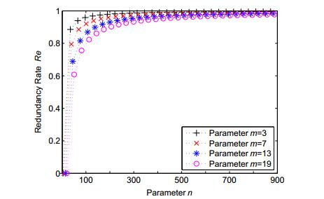
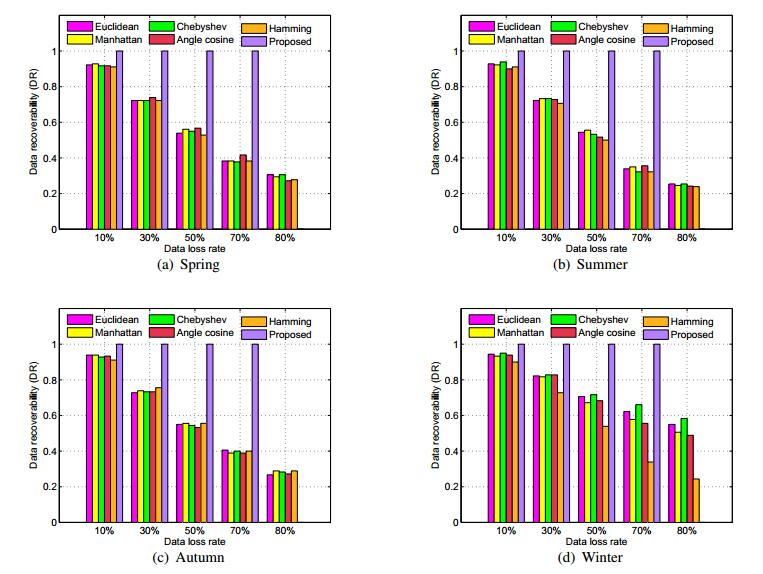
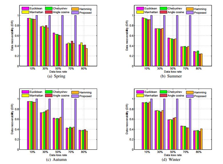
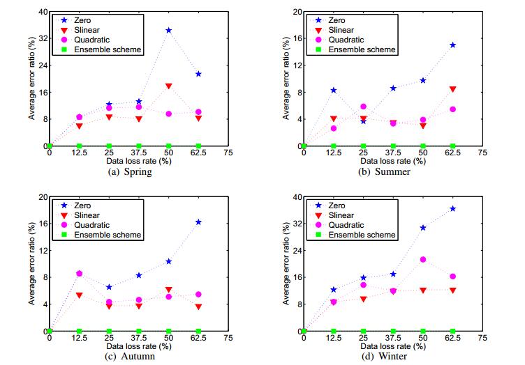
Figures(9)  /  Tables(4)

Other Articles By Authors

/

DownLoad:  Full-Size Img  PowerPoint
Return
Return

Catalog