The regression of mutually independent time series, whether stationary or non-stationary, will result in autocorrelation in the random error term. This leads to the over-rejection of the null hypothesis in the conventional t-test, causing spurious regression. We propose a new method to reduce spurious regression by applying the Cochrane-Orutt feasible generalized least squares method based on a bias-corrected method for a first-order autoregressive model in finite samples. This method eliminates the requirements for a kernel function and bandwidth selection, making it simpler to implement than the traditional heteroskedasticity and autocorrelation consistent method. A series of Monte Carlo simulations indicate that our method can decrease the probability of spurious regression among stationary, non-stationary, or trend-stationary series within a sample size of 10–50. We applied this proposed method to the actual data studied by Yule in 1926, and found that it can significantly minimize spurious regression. Thus, we deduce that there is no significant regressive relationship between the proportion of marriages in the Church of England and the mortality rate in England and Wales.
Citation: Zhongzhe Ouyang, Ke Liu, Min Lu. Bias correction based on AR model in spurious regression[J]. AIMS Mathematics, 2024, 9(4): 8439-8460. doi: 10.3934/math.2024410
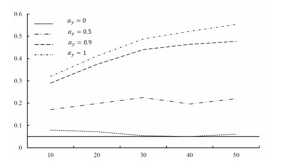
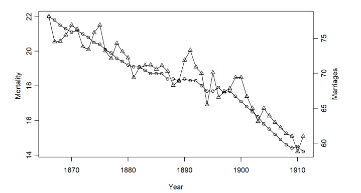
The regression of mutually independent time series, whether stationary or non-stationary, will result in autocorrelation in the random error term. This leads to the over-rejection of the null hypothesis in the conventional t-test, causing spurious regression. We propose a new method to reduce spurious regression by applying the Cochrane-Orutt feasible generalized least squares method based on a bias-corrected method for a first-order autoregressive model in finite samples. This method eliminates the requirements for a kernel function and bandwidth selection, making it simpler to implement than the traditional heteroskedasticity and autocorrelation consistent method. A series of Monte Carlo simulations indicate that our method can decrease the probability of spurious regression among stationary, non-stationary, or trend-stationary series within a sample size of 10–50. We applied this proposed method to the actual data studied by Yule in 1926, and found that it can significantly minimize spurious regression. Thus, we deduce that there is no significant regressive relationship between the proportion of marriages in the Church of England and the mortality rate in England and Wales.

| [1] |
G. U. Yule, Why do we sometimes get nonsense-correlations between time-series, J. Royal Stat. Soc., 89 (1926), 1–63. https://doi.org/10.1017/CBO9781139170116.012 doi: 10.1017/CBO9781139170116.012

|
| [2] |
Y. Wen, Y. Xu, Statistical monitoring of economic growth momentum transformation: empirical study of Chinese provinces, AIMS Math., 8 (2023), 24825–24847. https://doi.org/10.3934/math.20231266 doi: 10.3934/math.20231266
|
| [3] |
Z. Li, F. Zou, B. Mo, Does mandatory CSR disclosure affect enterprise total factor productivity, Econ. Res., 35 (2022), 4902–4921. https://doi.org/10.1080/1331677X.2021.2019596 doi: 10.1080/1331677X.2021.2019596
|
| [4] |
N. Stanojević, K. Zakić, China and deglobalization of the world economy, Natl. Account. Rev., 5 (2023), 67–85. https://doi.org/10.3934/NAR.2023005 doi: 10.3934/NAR.2023005
|
| [5] |
Y. Liu, Z. Li, M. Xu, The influential factors of financial cycle spillover: evidence from China, Emerg. Mark. Financ. Tr., 56 (2020), 1336–1350. https://doi.org/10.1080/1540496X.2019.1658076 doi: 10.1080/1540496X.2019.1658076
|
| [6] |
Z. Li, J. Zhong, Impact of economic policy uncertainty shocks on China's financial conditions, Financ. Res. Lett., 35 (2020), 101303. https://doi.org/10.1016/j.frl.2019.101303 doi: 10.1016/j.frl.2019.101303
|
| [7] |
Z. Li, B. Mo, H. Nie, Time and frequency dynamic connectedness between cryptocurrencies and financial assets in China, Int. Rev. Econ. Financ., 86 (2023), 46–57. https://doi.org/10.1016/j.iref.2023.01.015 doi: 10.1016/j.iref.2023.01.015
|
| [8] |
N. T. Giannakopoulos, D. P. Sakas, N. Kanellos, C. Christopoulos, Web analytics and supply chain transportation firms' financial performance, Natl. Account. Rev., 5 (2023), 405–420. https://doi.org/10.3934/NAR.2023023 doi: 10.3934/NAR.2023023
|
| [9] |
Z. Li, Z. Huang, H. Dong, The influential factors on outward foreign direct investment: evidence from the "the belt and road", Emerg. Mark. Financ. Tr., 55 (2019), 3211–3226. https://doi.org/10.1080/1540496X.2019.1569512 doi: 10.1080/1540496X.2019.1569512
|
| [10] |
M. Hong, J. He, K. Zhang, Z. Guo, Does digital transformation of enterprises help reduce the cost of equity capital, Math. Biosci. Eng., 20 (2023), 6498–6516. https://doi.org/10.3934/mbe.2023280 doi: 10.3934/mbe.2023280
|
| [11] |
Z. Li, J. Zhu, J. He, The effects of digital financial inclusion on innovation and entrepreneurship: a network perspective, Electron. Res. Arch., 30 (2022), 4740–4762. https://doi.org/10.3934/era.2022240 doi: 10.3934/era.2022240
|
| [12] |
Z. Li, H. Chen, B. Mo, Can digital finance promote urban innovation? Evidence from China, Borsa Istanb. Rev., 23 (2023), 285–296. https://doi.org/10.1016/j.bir.2022.10.006 doi: 10.1016/j.bir.2022.10.006
|
| [13] |
Z. Li, C. Yang, Z. Huang, How does the fintech sector react to signals from central bank digital currencies, Financ. Res. Lett., 50 (2022), 103308. https://doi.org/10.1016/j.frl.2022.103308 doi: 10.1016/j.frl.2022.103308
|
| [14] |
Y. Liu, L. Chen, H. Luo, Y. Liu, Y. Wen, The impact of intellectual property rights protection on green innovation: a quasi-natural experiment based on the pilot policy of the Chinese intellectual property court, Math. Biosci. Eng., 21 (2024), 2587–2607. https://doi.org/10.3934/mbe.2024114 doi: 10.3934/mbe.2024114
|
| [15] |
Y. Wang, J. Liu, X. Yang, M. Shi, R. Ran, The mechanism of green finance's impact on enterprises' sustainable green innovation, Green Financ., 5 (2023), 452–478. https://doi.org/10.3934/GF.2023018 doi: 10.3934/GF.2023018
|
| [16] |
J. Duan, T. Liu, X. Yang, H. Yang, Y. Gao, Financial asset allocation and green innovation, Green Financ., 5 (2023), 512–537. https://doi.org/10.3934/GF.2023020 doi: 10.3934/GF.2023020
|
| [17] |
Z. Li, Z. Huang, Y. Su, New media environment, environmental regulation and corporate green technology innovation: evidence from China, Energy Economics, 119 (2023), 106545. https://doi.org/10.1016/j.eneco.2023.106545 doi: 10.1016/j.eneco.2023.106545
|
| [18] |
S. K. Agyei, A. Bossman, Investor sentiment and the interdependence structure of GIIPS stock market returns: a multiscale approach, Quant. Financ. Econ., 7 (2023), 87–116. https://doi.org/10.3934/QFE.2023005 doi: 10.3934/QFE.2023005
|
| [19] |
J. Saleemi, Political-obsessed environment and investor sentiments: pricing liquidity through the microblogging behavioral perspective, Data Sci. Financ. Econ., 3 (2023), 196–207. https://doi.org/10.3934/DSFE.2023012 doi: 10.3934/DSFE.2023012
|
| [20] |
T. C. Chiang, Stock returns and inflation expectations: evidence from 20 major countries, Quant. Financ. Econ., 7 (2023), 538–568. https://doi.org/10.3934/QFE.2023027 doi: 10.3934/QFE.2023027
|
| [21] |
C. Granger, N. Hyung, Y. Jeon, Spurious regression with stationary series, Appl. Econ., 33 (2001), 899–904. https://doi.org/10.1080/00036840121734 doi: 10.1080/00036840121734
|
| [22] |
C. Granger, P. Newbold, Spurious regressions in econometrics, J. Econometrics, 2 (1974), 111–120. https://doi.org/10.1016/0304-4076(74)90034-7 doi: 10.1016/0304-4076(74)90034-7
|
| [23] |
T. H. Kim, Y. S. Lee, P. Newbold, Spurious regressions with stationary processes around linear trends, Econ. Lett., 83 (2004), 257–262. https://doi.org/10.1016/j.econlet.2003.10.020 doi: 10.1016/j.econlet.2003.10.020
|
| [24] |
D. Ventosa-Santaulária, Spurious regression, J. Probab. Stat., 2009 (2009), 1–27. https://doi.org/10.1155/2009/802975 doi: 10.1155/2009/802975
|
| [25] |
H. Liu, The analysis of spurious regressions instationary processes without drifts, J. Quant. Tech. Econ., 27 (2010), 142–154. https://doi.org/10.13653/j.cnki.jqte.2010.11.001 doi: 10.13653/j.cnki.jqte.2010.11.001
|
| [26] |
B. T. McCallum, Is the spurious regression problem spurious, Econ. Lett., 107 (2010), 321–323. https://doi.org/10.1016/j.econlet.2010.02.004 doi: 10.1016/j.econlet.2010.02.004
|
| [27] |
H. Liu, A study on the properties and correction of HAC method and its application in the spurious regression, J. Quant. Tech. Econ., 32 (2015), 148–161. https://doi.org/10.13653/j.cnki.jqte.2015.11.010 doi: 10.13653/j.cnki.jqte.2015.11.010
|
| [28] |
H. Liu, C. Li, Application of bias-correction prewhitening HAC methods in the spurious regression, J. Quant. Tech. Econ., 30 (2013), 109–123. https://doi.org/10.13653/j.cnki.jqte.2013.08.021 doi: 10.13653/j.cnki.jqte.2013.08.021
|
| [29] |
C. Y. Choi, L. Hu, M. Ogaki, Robust estimation for structural spurious regressions and a Hausman-type cointegration test, J. Econometrics, 142 (2008), 327–351. https://doi.org/10.1016/j.jeconom.2007.06.003 doi: 10.1016/j.jeconom.2007.06.003
|
| [30] |
M. Wu, Fgls method based on finite samples, J. Quant. Tech. Econ., 30 (2013), 148–160. https://doi.org/10.13653/j.cnki.jqte.2013.07.022 doi: 10.13653/j.cnki.jqte.2013.07.022
|
| [31] |
S. H. Sørbye, P. G. Nicolau, H. Rue, Finite-sample properties of estimators for first and second order autoregressive processes, Stat. Infer. Stoch. Pro., 25 (2022), 577–598. https://doi.org/10.1007/s11203-021-09262-4 doi: 10.1007/s11203-021-09262-4
|
| [32] |
J. H. Kim, Forecasting autoregressive time series with bias-corrected parameter estimators, Int. J. Forecast., 19 (2003), 493–503. https://doi.org/10.1016/S0169-2070(02)00062-6 doi: 10.1016/S0169-2070(02)00062-6
|
| [33] | S. Wang, J. Hu, Trend-cycle decomposition and stochastic impact effect of Chinese GDP, Econ. Res. J., 44 (2009), 65–76. |
| [34] |
A. E. Noriega, D. Ventosa-Santaulária, Spurious regression and trending variables, Oxford Bull. Econ. Stat., 69 (2007), 439–444. https://doi.org/10.1111/j.1468-0084.2007.00481.x doi: 10.1111/j.1468-0084.2007.00481.x
|
| [35] |
L. García-Belmonte, D. Ventosa-Santaulária, Spurious regression and lurking variables, Stat. Probab. Lett., 81 (2011), 2004–2010. https://doi.org/10.1016/j.spl.2011.08.015 doi: 10.1016/j.spl.2011.08.015
|
| [36] |
M. Wu, P. You, Solution of spurious regression with trending variables, J. Quant. Tech. Econ., 12 (2016), 113–128. https://doi.org/10.13653/j.cnki.jqte.2016.12.007 doi: 10.13653/j.cnki.jqte.2016.12.007
|
| [37] |
C. S. H. Wang, C. M. Hafner, A simple solution of the spurious regressionproblem, Stud. Nonlinear Dyn. Econ., 22 (2018), 1–14. https://doi.org/10.1515/snde-2015-0040 doi: 10.1515/snde-2015-0040
|
| [38] |
C. Kao, Spurious regression and residual-based testsfor cointegration in panel data, J. Econometrics, 90 (1999), 1–44. https://doi.org/10.1016/S0304-4076(98)00023-2 doi: 10.1016/S0304-4076(98)00023-2
|
| [39] |
A. Onatski, C. Wang, Spurious factor analysis, Econometrica, 89 (2021), 591–614. https://doi.org/10.3982/ECTA16703 doi: 10.3982/ECTA16703
|
| [40] |
M. Khumalo, H. Mashele, M. Seitshiro, Quantification of the stock market value at risk by using fiaparch, hygarch and figarch models, Data Sci. Financ. Econ., 3 (2023), 380–400. https://doi.org/10.3934/DSFE.2023022 doi: 10.3934/DSFE.2023022
|
Figures(2) / Tables(7)

Zhongzhe Ouyang, Ke Liu, Min Lu. Bias correction based on AR model in spurious regression[J]. AIMS Mathematics, 2024, 9(4): 8439-8460. doi: 10.3934/math.2024410


 DownLoad: