In the field of higher education, the transition from secondary to tertiary education is crucial to reduce dropout rates and to improve the educational outcomes. This study aims to investigate various predictors that affect the academic performance of first-year Business Administration and Management (BAM) students, thereby emphasizing the importance of mathematical literacy. Using a structural equation modeling approach, this investigation looks beyond gender to include baccalaureate choices such as the mathematics pathway and the mathematics entrance exam grades. This study adopts a comprehensive approach by using administrative data from a public university in an outermost region with economic resources and academic performance below the national average. Starting with bivariate descriptive analyses, it moves on to multivariate analyses through structural equation models, thereby examining the joint correlation of variables related to mathematical literacy with the construct 'academic success' in the first year of BAM. The results reveal a dual mediating effect on women's academic success through the chosen mathematics pathway and the grades obtained in the mathematics entrance examination. The study demonstrates a significant correlation between mathematical literacy and academic success in the first year of the BAM degree, both in the subjects with a mathematical component and in those with a higher theoretical component, thus highlighting statistical gender differences. These findings underscore the need for a broader focus beyond gender, including baccalaureate choices in the analysis, to improve the predictions and interventions aimed at enhancing academic success in BAM programs.
Citation: Inmaculada Galván-Sánchez, Alexis J. López-Puig, Margarita Fernández-Monroy, Sara M. González-Betancor. The mediating role of mathematical literacy in first-year educational outcomes in Business Administration and Management degrees: A gender-based analysis[J]. AIMS Mathematics, 2024, 9(11): 29974-29999. doi: 10.3934/math.20241448
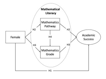
In the field of higher education, the transition from secondary to tertiary education is crucial to reduce dropout rates and to improve the educational outcomes. This study aims to investigate various predictors that affect the academic performance of first-year Business Administration and Management (BAM) students, thereby emphasizing the importance of mathematical literacy. Using a structural equation modeling approach, this investigation looks beyond gender to include baccalaureate choices such as the mathematics pathway and the mathematics entrance exam grades. This study adopts a comprehensive approach by using administrative data from a public university in an outermost region with economic resources and academic performance below the national average. Starting with bivariate descriptive analyses, it moves on to multivariate analyses through structural equation models, thereby examining the joint correlation of variables related to mathematical literacy with the construct 'academic success' in the first year of BAM. The results reveal a dual mediating effect on women's academic success through the chosen mathematics pathway and the grades obtained in the mathematics entrance examination. The study demonstrates a significant correlation between mathematical literacy and academic success in the first year of the BAM degree, both in the subjects with a mathematical component and in those with a higher theoretical component, thus highlighting statistical gender differences. These findings underscore the need for a broader focus beyond gender, including baccalaureate choices in the analysis, to improve the predictions and interventions aimed at enhancing academic success in BAM programs.

| [1] |
L. Kemper, G. Vorhoff, B. U. Wigger, Predicting student dropout: A machine learning approach, Eur. J. High. Educ., 10 (2020), 28–47. https://doi.org/10.1080/21568235.2020.1718520 doi: 10.1080/21568235.2020.1718520

|
| [2] | Ministerio de Universidades, Datos y cifras del Sistema Universitario Español. Publicación 2022-2023, Madrid, Spain, 2023. Available from: https://www.universidades.gob.es/wp-content/uploads/2023/04/DyC_2023_web_v2.pdf. |
| [3] | J. Hernández Armenteros, J.A. Pérez García, La universidad española en cifras, 2019/2020, CRUE Universidades Españolas, 2023. Available from: https://www.crue.org/wp-content/uploads/2023/04/CRUE_UEC_22_1-PAG.pdf. |
| [4] | Ministerio de Universidades, Datos y cifras del Sistema Universitario Español. Publicación 2019-2020, 2020. Available from: https://www.universidades.gob.es/wp-content/uploads/2022/10/Datos_y_Cifras_2019-2020.pdf. |
| [5] |
P. R. Bahr, Does mathematics remediation work?: A comparative analysis of academic attainment among community college students, Res. High. Educ., 49 (2008), 420–450. https://doi.org/10.1007/s11162-008-9089-4 doi: 10.1007/s11162-008-9089-4
|
| [6] |
M. Fernández-Mellizo, A. Constante-Amores, Factors associated to the academic performance of new entry students at Complutense University of Madrid, Revista de Educación, 387 (2020), 213–240. https://doi.org/10.4438/1988-592X-RE-2020-387-433 doi: 10.4438/1988-592X-RE-2020-387-433
|
| [7] |
S. S. El Massah, D. Fadly, Predictors of academic performance for finance students: Women at higher education in the UAE, Int. J. Edu. Manag., 31 (2017), 854–864. https://doi.org/10.1108/IJEM-12-2015-0171 doi: 10.1108/IJEM-12-2015-0171
|
| [8] |
A. Laging, R. Voßkamp, Determinants of maths performance of first-year Business Administration and Economics students, Int. J. Res. Undergrad. Math. Educ., 3 (2017), 108–142. https://doi.org/10.1007/s40753-016-0048-8 doi: 10.1007/s40753-016-0048-8
|
| [9] |
N. Eather, M. F. Mavilidi, H. Sharp, R. Parkes, Programmes targeting student retention/success and satisfaction/experience in higher education: A systematic review, J. High. Educ. Policy Manag., 44 (2022), 223–239. https://doi.org/10.1080/1360080X.2021.2021600 doi: 10.1080/1360080X.2021.2021600
|
| [10] |
K. McKenzie, R. Schweitzer, Who succeeds at university? Factors predicting academic performance in first year Australian university students, High. Educ. Res. Dev., 20 (2001), 21–33. https://doi.org/10.1080/07924360120043621 doi: 10.1080/07924360120043621
|
| [11] |
R. McNabb, S. Pal, P. Sloane, Gender differences in educational attainment: The case of university students in England and Wales, Economica, 69 (2002), 481–503. https://doi.org/10.1111/1468-0335.00295 doi: 10.1111/1468-0335.00295
|
| [12] |
E. Smith, P. White, What makes a successful undergraduate? the relationship between student characteristics, degree subject and academic success at university, Br. Educ. Res. J., 41 (2015), 686–708. https://doi.org/10.1002/berj.3158 doi: 10.1002/berj.3158
|
| [13] |
C. Castagnetti, L. Rosti, Effort allocation in tournaments: The effect of gender on academic performance in Italian universities, Econ. Educ. Rev., 28 (2009), 357–369. https://doi.org/10.1016/j.econedurev.2008.06.004 doi: 10.1016/j.econedurev.2008.06.004
|
| [14] |
T. Thiele, A. Singleton, D. Pope, D. Stanistreet, Predicting students' academic performance based on school and socio-demographic characteristics, Stud. High. Educ., 41 (2016), 1424–1446. https://doi.org/10.1080/03075079.2014.974528 doi: 10.1080/03075079.2014.974528
|
| [15] |
R. Asian-Chaves, E. M. Buitrago, I. Masero-Moreno, R. Yñiguez, Advanced mathematics: An advantage for business and management administration students, Int. J. Manag. Educ., 19 (2021), 100498. https://doi.org/10.1016/j.ijme.2021.100498 doi: 10.1016/j.ijme.2021.100498
|
| [16] |
J.B. Horowitz, L. Spector, Is there a difference between private and public education on college performance? Econ. Educ. Rev., 24 (2005), 189–195. https://doi.org/10.1016/j.econedurev.2004.03.007 doi: 10.1016/j.econedurev.2004.03.007
|
| [17] |
K. Danilowicz-Gösele, K. Lerche, J. Meya, R. Schwager, Determinants of students' success at university, Educ. Econ., 25 (2017), 513–532. https://doi.org/10.1080/09645292.2017.1305329 doi: 10.1080/09645292.2017.1305329
|
| [18] |
C. Teixeira, D. Gomes, J. Borges, Introductory accounting students' motives, expectations and Preparedness for Higher Education: Some Portuguese evidence, Account. Educ., 24 (2015), 123–145. https://doi.org/10.1080/09639284.2015.1018284 doi: 10.1080/09639284.2015.1018284
|
| [19] |
R. Woodfield, D. Jessop, L. McMillan, Gender differences in undergraduate attendance rates, Stud. High. Educ., 31 (2006), 1–22. https://doi.org/10.1080/03075070500340127 doi: 10.1080/03075070500340127
|
| [20] |
E. Totty, High school value-added and college outcomes, Educ. Econ., 28 (2020), 67–95. https://doi.org/10.1080/09645292.2019.1676880 doi: 10.1080/09645292.2019.1676880
|
| [21] |
S. M. Lindberg, J. S. Hyde, J. L. Petersen, M. C. Linn, New trends in gender and mathematics performance: A meta-analysis, Psychol. Bull., 136 (2010), 1123–1135. https://doi.org/10.1037/a0021276.supp doi: 10.1037/a0021276.supp
|
| [22] |
I. J. M. Arnold, J. T. Straten, Motivation and math skills as determinants of first-year performance in economics, J. Econ. Educ., 43 (2012), 33–47. https://doi.org/10.1080/00220485.2012.636709 doi: 10.1080/00220485.2012.636709
|
| [23] |
S. M. González-Betancor, M. Fernández-Monroy, I. Galván-Sánchez, A. J. López-Puig, Academic performance of first-year university students: Modelling the role of reading competence, High. Educ. Res. & Dev., 42 (2023), 1422–1437. https://doi.org/10.1080/07294360.2022.2142534 doi: 10.1080/07294360.2022.2142534
|
| [24] |
I. J. M. Arnold, W. Rowaan, First-year study success in economics and econometrics: The role of gender, motivation, and math skills, J. Econ. Educ., 45 (2014), 25–35. https://doi.org/10.1080/00220485.2014.859957 doi: 10.1080/00220485.2014.859957
|
| [25] | M. Hodara, K. Lewis, How well does high school grade point average predict college performance by student urbanicity and timing of college entry? Regional Educational Laboratory Northwest, 2017. Available from: https://ies.ed.gov/ncee/edlabs/projects/project.asp?projectID = 4546. |
| [26] |
R. Asian Chaves, E. M. Buitrago Esquinas, I. Masero, R. Yñíguez Ovando, Mathematical background as a success factor in Economics and Business degrees, CSR, 24 (2022), 758–772. https://doi.org/10.1177/1521025120946452 doi: 10.1177/1521025120946452
|
| [27] |
J. M. Cerdeira, L. C. Nunes, A. B. Reis, C. Seabra, Predictors of student success in Higher Education: Secondary school internal scores versus national exams, High. Educ. Quart., 72 (2018), 304–313. https://doi.org/10.1111/hequ.12158 doi: 10.1111/hequ.12158
|
| [28] |
P. L. Silva, L. C. Nunes, C. Seabra, A. B. Reis, M. Alves, Student selection and performance in higher education: admission exams vs. high school scores, Educ. Econ., 28 (2020), 437–454. https://doi.org/10.1080/09645292.2020.1782846 doi: 10.1080/09645292.2020.1782846
|
| [29] |
J. T. E. Richardson, A. Woodley, Another look at the role of age, gender and subject as predictors of academic attainment in Higher Education, Stud. High. Educ., 28 (2003), 475–493. https://doi.org/10.1080/0307507032000122305 doi: 10.1080/0307507032000122305
|
| [30] |
E. Ní Fhloinn, O. Fitzmaurice, C. Mac an Bhaird, C. O'Sullivan, Student perception of the impact of mathematics support in higher education, Int. J. Math. Educ. Sci. Technol., 45 (2014), 953–967. https://doi.org/10.1080/0020739X.2014.892161 doi: 10.1080/0020739X.2014.892161
|
| [31] | G. C. Leder, Gender and mathematics education: An overview, In: Compendium for Early Career Researchers in Mathematics Education, Springer: Cham, 2019,289–308. https://doi.org/10.1007/978-3-030-15636-7_13 |
| [32] |
S. Rossi, I. Xenidou-Dervou, E. Simsek, C. Artemenko, G. Daroczy, H. C. Nuerk, et al., Mathematics–gender stereotype endorsement influences mathematics anxiety, self-concept, and performance differently in men and women, Ann. N. Y. Acad. Sci., 1513 (2022), 121–139. https://doi.org/10.1111/nyas.14779 doi: 10.1111/nyas.14779
|
| [33] |
K. Eriksson, T. Lindholm, Making gender matter: The role of gender-based expectancies and gender identification on women's and men's math performance in Sweden: Personality and Social Sciences, Scand. J. Psychol., 48 (2007), 329–338. https://doi.org/10.1111/j.1467-9450.2007.00588.x doi: 10.1111/j.1467-9450.2007.00588.x
|
| [34] |
H. J. Johnson, L. Barnard-Brak, T. F. Saxon, M. K. Johnson, An experimental study of the effects of stereotype threat and stereotype lift on men and women's performance in mathematics, J. Exp. Educ., 80 (2012), 137–149. https://doi.org/10.1080/00220973.2011.567312 doi: 10.1080/00220973.2011.567312
|
| [35] |
L. T. O'Brien, C. S. Crandall, Stereotype threat and arousal: Effects on women's math performance, Pers. Soc. Psychol. Bull., 29 (2003), 782–789. https://doi.org/10.1177/0146167203029006010 doi: 10.1177/0146167203029006010
|
| [36] |
D. Contini, M. L. Di Tommaso, S. Mendolia, The gender gap in mathematics achievement: Evidence from Italian data, Econ. Educ. Rev., 58 (2017), 32–42. https://doi.org/10.1016/j.econedurev.2017.03.001 doi: 10.1016/j.econedurev.2017.03.001
|
| [37] |
Z. Salikutluk, S. Heyne, Do gender roles and norms affect performance in maths? The impact of adolescents' and their peers' gender conceptions on maths grades, Eur. Sociol. Rev., 33 (2017), 368–381. https://doi.org/10.1093/esr/jcx049 doi: 10.1093/esr/jcx049
|
| [38] |
E. De Gioannis, The conundrum of gender-science stereotypes: A review and discussion of measurements, Qual. Quant., 57 (2023), 3165–3182. https://doi.org/10.1007/s11135-022-01512-8 doi: 10.1007/s11135-022-01512-8
|
| [39] |
J. L. Arroyo-Barrigüete, S. C. López, A. Hernández, M. Segura, Effect of advanced high school major on mathematical performance at university: A comparative study in Business Administration degrees, Revista de Educacion, 1 (2023), 115–140. https://doi.org/10.4438/1988-592X-RE-2023-402-597 doi: 10.4438/1988-592X-RE-2023-402-597
|
| [40] |
J. Alcock, S. Cockcroft, F. Finn, Quantifying the advantage of secondary mathematics study for accounting and finance undergraduates, Account. Financ., 48 (2008), 697–718. https://doi.org/10.1111/j.1467-629X.2008.00261.x doi: 10.1111/j.1467-629X.2008.00261.x
|
| [41] |
L. Opstad, Success in business studies and mathematical background: The case of Norway, J. Appl. Res. High. Educ., 10 (2018), 399–408. https://doi.org/10.1108/JARHE-11-2017-0136 doi: 10.1108/JARHE-11-2017-0136
|
| [42] |
J. Sikora, D. G. W. Pitt, Does advanced mathematics help students enter university more than basic mathematics? Gender and returns to year 12 mathematics in Australia, Math. Educ. Res. J., 31 (2019), 197–218. https://doi.org/10.1007/s13394-018-0249-3 doi: 10.1007/s13394-018-0249-3
|
| [43] |
C. Mills, J. Heyworth, L. Rosenwax, S. Carr, M. Rosenberg, Factors associated with the academic success of first year Health Science students, Adv. Health Sci. Educ., 14 (2009), 205–217. https://doi.org/10.1007/s10459-008-9103-9 doi: 10.1007/s10459-008-9103-9
|
| [44] |
C. F. Rodríguez-Hernández, E. Cascallar, E. Kyndt, Socio-economic status and academic performance in higher education: A systematic review, Educ. Res. Rev., 29 (2020), 100305. https://doi.org/10.1016/j.edurev.2019.100305 doi: 10.1016/j.edurev.2019.100305
|
| [45] |
Z. Li, B. Chen, S. Lu, The impact of information and communication technology on financial inclusion-based on a global perspective, AIMS Mathematics, 7 (2022), 20930–20961. https://doi.org/10.3934/math.20221147 doi: 10.3934/math.20221147
|
| [46] |
G. S. Black, A. L. Schofield, A comparative study of the determinants of future plans and expectations of business students, J. Educ. Bus., 93 (2018), 75–87. https://doi.org/10.1080/08832323.2018.1424109 doi: 10.1080/08832323.2018.1424109
|
| [47] |
J. L. Arroyo-Barrigüete, S. Carabias-López, F. Borrás-Pala, G. Martín-Antón, Gender Differences in Mathematics Achievement: The Case of a Business School in Spain, Sage Open, 13 (2023). https://doi.org/10.1177/21582440231166922 doi: 10.1177/21582440231166922
|
| [48] |
P. Kotlikoff, A. S. Rahman, K. A. Smith, Minding the gap: Academic outcomes from pre-college programs, Educ. Econ., 30 (2022), 3–28. https://doi.org/10.1080/09645292.2021.1931664 doi: 10.1080/09645292.2021.1931664
|


Figures(4) / Tables(6)

Inmaculada Galván-Sánchez, Alexis J. López-Puig, Margarita Fernández-Monroy, Sara M. González-Betancor. The mediating role of mathematical literacy in first-year educational outcomes in Business Administration and Management degrees: A gender-based analysis[J]. AIMS Mathematics, 2024, 9(11): 29974-29999. doi: 10.3934/math.20241448


 DownLoad: