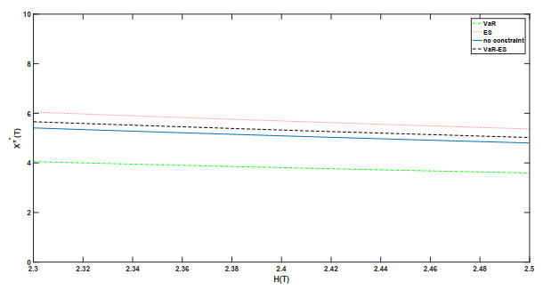
In this paper, we investigated an optimal investment problem of a defined contribution (DC) pension plan under a joint Value-at-Risk (VaR) and an expected shortfall (ES) constraint. By using a martingale method, we transformed a dynamic optimization problem to a static pointwise optimization problem and derived the closed-form representations of the optimal wealth and portfolio processes in terms of the state price density. Numerical results showed that in comparison to only an ES constraint or a VaR constraint, the joint VaR-ES constraint can not only improve risk management for the bad economic states but also lower the volatility of the optimal terminal wealth.
Citation: Yinghui Dong, Chengjin Tang, Chunrong Hua. Optimal investment of DC pension plan under a joint VaR-ES constraint[J]. AIMS Mathematics, 2024, 9(1): 2084-2104. doi: 10.3934/math.2024104
In this paper, we investigated an optimal investment problem of a defined contribution (DC) pension plan under a joint Value-at-Risk (VaR) and an expected shortfall (ES) constraint. By using a martingale method, we transformed a dynamic optimization problem to a static pointwise optimization problem and derived the closed-form representations of the optimal wealth and portfolio processes in terms of the state price density. Numerical results showed that in comparison to only an ES constraint or a VaR constraint, the joint VaR-ES constraint can not only improve risk management for the bad economic states but also lower the volatility of the optimal terminal wealth.

| [1] |
G. Deelstra, M. Grasselli, P. F. Koehl, Optimal design of the guarantee for defined contribution funds, J. Econ. Dyn. Control, 28 (2004), 2239–2260. https://doi.org/10.1016/j.jedc.2003.10.003 doi: 10.1016/j.jedc.2003.10.003

|
| [2] |
D. Blake, D. Wright, Y. Zhang, Age-dependent investing: Optimal funding and investment strategies in defined contribution pension plans when members are rational life cycle financial planners, J. Econ. Dyn. Control, 38 (2014), 105–124. https://doi.org/10.1016/j.jedc.2013.11.001 doi: 10.1016/j.jedc.2013.11.001
|
| [3] |
J. Gao, Optimal portfolios for DC pension plans under a CEV model, Insur. Math. Econ., 44 (2009), 479–490. https://doi.org/10.1016/j.insmatheco.2009.01.005 doi: 10.1016/j.insmatheco.2009.01.005
|
| [4] |
E. Vigna, S. Haberman, Optimal investment strategy for defined contribution pension schemes, Insur. Math. Econ., 28 (2001), 233–262. https://doi.org/10.1016/S0167-6687(00)00077-9 doi: 10.1016/S0167-6687(00)00077-9
|
| [5] |
S. Haberman, E. Vigna, Optimal investment strategies and risk measures in defined contribution pension schemes, Insur. Math. Econ., 31 (2002), 35–69. https://doi.org/10.1016/S0167-6687(02)00128-2 doi: 10.1016/S0167-6687(02)00128-2
|
| [6] |
Y. Zeng, D. P. Li, Z. Chen, Z. Yang, Ambiguity aversion and optimal derivative-based pension investment with stochastic income and volatility, J. Econ. Dyn. Control, 88 (2018), 70–103. https://doi.org/10.1016/j.jedc.2018.01.023 doi: 10.1016/j.jedc.2018.01.023
|
| [7] |
L. Zhang, H. Zhang, H. X. Yao, Optimal investment management for a defined contribution pension fund under imperfect information, Insur. Math. Econ., 79 (2018), 210–224. https://doi.org/10.1016/j.insmatheco.2018.01.007 doi: 10.1016/j.insmatheco.2018.01.007
|
| [8] |
A. J. G. Cairns, D. Blake, K. Dowd, Stochastic lifestyling: Optimal dynamic asset allocation for defined contribution pension plans, J. Econ. Dyn. Control, 30 (2006), 843–877. https://doi.org/10.1016/j.jedc.2005.03.009 doi: 10.1016/j.jedc.2005.03.009
|
| [9] |
H. X. Yao, Z. Yang, P. Chen, Markowitz's mean-variance defined contribution pension fund management under inflation: A continuous-time model, Insur. Math. Econ., 53 (2013), 851–863. https://doi.org/10.1016/j.insmatheco.2013.10.002 doi: 10.1016/j.insmatheco.2013.10.002
|
| [10] |
G. H. Guan, Z. X. Liang, Optimal management of DC pension plan in a stochastic interest rate and stochastic volatility framework, Insur. Math. Econ., 57 (2014), 58–66. https://doi.org/10.1016/j.insmatheco.2014.05.004 doi: 10.1016/j.insmatheco.2014.05.004
|
| [11] |
P. Wang, Z. F. Li, J. Y. Sun, Robust portfolio choice for a DC pension plan with inflation risk and mean-reverting risk premium under ambiguity, Optimization, 70 (2021), 191–224. https://doi.org/10.1080/02331934.2019.1679812 doi: 10.1080/02331934.2019.1679812
|
| [12] |
A. H. Zhang, R. Korn, C. O. Ewald, Optimal management and inflation protection for defined contribution pension plans, Blatter DGVFM., 28 (2007), 239–258. https://doi.org/10.1007/s11857-007-0019-x doi: 10.1007/s11857-007-0019-x
|
| [13] |
J. F. Boulier, S. J. Huang, G. Taillard, Optimal management under stochastic interest rates: the case of a protected defined contribution pension fund, Insur. Math. Econ., 28 (2001), 173–189. https://doi.org/10.1016/S0167-6687(00)00073-1 doi: 10.1016/S0167-6687(00)00073-1
|
| [14] |
J. Y. Sun, Y. J. Li, L. Zhang, Robust portfolio choice for a defined contribution pension plan with stochastic income and interest rate, Commun. Stat.-Theor. M., 47 (2018), 4106–4130. https://doi.org/10.1080/03610926.2017.1367815 doi: 10.1080/03610926.2017.1367815
|
| [15] |
G. H. Guan, Z. X. Liang, Optimal management of DC pension plan under loss aversion and Value-at-Risk constraints, Insur. Math. Econ., 69 (2016), 224–237. https://doi.org/10.1016/j.insmatheco.2016.05.014 doi: 10.1016/j.insmatheco.2016.05.014
|
| [16] |
Y. H. Dong, H. Zheng, Optimal investment with S-shaped utility and trading and Value at Risk constraints: An application to defined contribution pension plan, Eur. J. Oper. Res., 281 (2020), 346–356. https://doi.org/10.1016/j.ejor.2019.08.034 doi: 10.1016/j.ejor.2019.08.034
|
| [17] |
S. Basak, A. Shapiro, Value-at-Risk-based risk management: Optimal policies and asset prices, Rev. Financ. Stud., 14 (2001), 371–405. https://doi.org/10.1093/rfs/14.2.371 doi: 10.1093/rfs/14.2.371
|
| [18] |
S. Basak, A general equilibrium model of portfolio insurance, Rev. Financ. Stud., 8 (1995), 1059–1090. https://doi.org/10.1093/rfs/8.4.1059 doi: 10.1093/rfs/8.4.1059
|
| [19] |
Y. H. Dong, H. Zheng, Optimal investment of DC pension plan under short-selling constraints and portfolio insurance, Insur. Math. Econ., 85 (2019), 47–59. https://doi.org/10.1016/j.insmatheco.2018.12.005 doi: 10.1016/j.insmatheco.2018.12.005
|
| [20] |
A. Chen, T. Nguyen, M. Stadje, Optimal investment under VaR-regulation and minimum insurance, Insur. Math. Econ., 79 (2018), 194–209. https://doi.org/10.1016/j.insmatheco.2018.01.008 doi: 10.1016/j.insmatheco.2018.01.008
|
| [21] | H. Mi, Z. Q. Xu, D. F. Yang, Optimal management of DC pension plan with inflation risk and tail VaR constraint, arXiv. preprint, 2023, https://doi.org/10.48550/arXiv.2309.01936 |
| [22] |
F. Y. Zhang, Non-concave portfolio optimization with average Value-at-Risk, Math. Finan. Econ., 17 (2023), 203–237. https://doi.org/10.1007/s11579-023-00332-0 doi: 10.1007/s11579-023-00332-0
|
| [23] |
P. Y. Wei, Risk management with expected shortfall, Math. Finan. Econ., 15 (2021), 847–883. https://doi.org/10.1007/s11579-021-00298-x doi: 10.1007/s11579-021-00298-x
|
| [24] |
Z. Chen, Z. F. Li, Y. Zeng, J. Y. Sun, Asset allocation under loss aversion and minimum performance constraint in a DC pension plan with inflation risk, Insur. Math. Econ., 75 (2017), 137–150. https://doi.org/10.1016/j.insmatheco.2017.05.009 doi: 10.1016/j.insmatheco.2017.05.009
|
| [25] |
L. He, Z. X. Liang, Y. Liu, M. Ma, Optimal control of DC pension plan management under two incentive schemes, N. Am. Actuar. J., 23 (2019), 120–141. https://doi.org/10.1080/10920277.2018.1513371 doi: 10.1080/10920277.2018.1513371
|

Figures(2) / Tables(2)

Yinghui Dong, Chengjin Tang, Chunrong Hua. Optimal investment of DC pension plan under a joint VaR-ES constraint[J]. AIMS Mathematics, 2024, 9(1): 2084-2104. doi: 10.3934/math.2024104


 DownLoad: