Uncertain multi-objective dynamic weapon-target allocation problem based on uncertainty theory

Guangjian Li; Guangjun He; Mingfa Zheng; Aoyu Zheng; Guangjian Li; Guangjun He; Mingfa Zheng; Aoyu Zheng

doi:10.3934/math.2023284

AIMS Mathematics

2023, Volume 8, Issue 3: 5639-5669. doi: 10.3934/math.2023284

Previous Article Next Article

Research article Special Issues

Uncertain multi-objective dynamic weapon-target allocation problem based on uncertainty theory

1.
Air Defense and Anti-missile School, Air Force Engineering University, Xi'an 710051, China
2.
Fundamentals Department, Air Force Engineering University, Xi'an 710051, China
3.
Equipment Management and Unmanned Aerial Vehicle Engineering School, Air Force Engineering University, Xi'an 710051, China

Received: 22 October 2022 Revised: 29 November 2022 Accepted: 12 December 2022 Published: 21 December 2022
MSC : 68U99

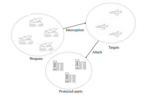
The weapon-target allocation (WTA) problem is a fundamental subject of defense-related applications research, and previous studies assume that the parameters in the model are determinate. For the real battlefield, asymmetric information usually leads to the failure of the above assumption, and there are uncertain factors whose frequency is hard to pinpoint. Based on uncertainty theory, we study a WTA problem in indeterminate battlefield in this paper. First, we analyze the uncertain factors in indeterminate battlefield and their influence on WTA problem. Then, considering the target threat value, the protected asset value and the extra cost of interception as uncertain variables, the uncertain multi-objective dynamic WTA (UMDWTA) model is established, where three indices including the value of destruction of targets, the value of surviving assets and the cost of operation are regarded as objective functions, and on this basis, an equivalent transformation is presented to convert the UMDWTA model into a determinate multi-objective programming (MOP) problem by expected value and standard deviation principle. To solve the proposed model efficiently, an improved multi-objective evolutionary algorithm based on decomposition (MOEA/D) is designed, which employs three new evolutionary operators and the weight vectors adaptation mechanism to improve the convergence and uniformity of the Pareto front obtained. Finally, a case of the UMDWTA problem is carried out to be solved by the designed algorithm, and the results verify the feasibility of the proposed model.
- uncertainty theory,
- weapon-target allocation,
- multi-objective programming,
- evolutionary algorithm
Citation: Guangjian Li, Guangjun He, Mingfa Zheng, Aoyu Zheng. Uncertain multi-objective dynamic weapon-target allocation problem based on uncertainty theory[J]. AIMS Mathematics, 2023, 8(3): 5639-5669. doi: 10.3934/math.2023284

Related Papers:

Abstract

The weapon-target allocation (WTA) problem is a fundamental subject of defense-related applications research, and previous studies assume that the parameters in the model are determinate. For the real battlefield, asymmetric information usually leads to the failure of the above assumption, and there are uncertain factors whose frequency is hard to pinpoint. Based on uncertainty theory, we study a WTA problem in indeterminate battlefield in this paper. First, we analyze the uncertain factors in indeterminate battlefield and their influence on WTA problem. Then, considering the target threat value, the protected asset value and the extra cost of interception as uncertain variables, the uncertain multi-objective dynamic WTA (UMDWTA) model is established, where three indices including the value of destruction of targets, the value of surviving assets and the cost of operation are regarded as objective functions, and on this basis, an equivalent transformation is presented to convert the UMDWTA model into a determinate multi-objective programming (MOP) problem by expected value and standard deviation principle. To solve the proposed model efficiently, an improved multi-objective evolutionary algorithm based on decomposition (MOEA/D) is designed, which employs three new evolutionary operators and the weight vectors adaptation mechanism to improve the convergence and uniformity of the Pareto front obtained. Finally, a case of the UMDWTA problem is carried out to be solved by the designed algorithm, and the results verify the feasibility of the proposed model.

References

[1]	A. S. Manne, A target assignment problem, Oper. Res., 6 (1958), 346–351. https://doi.org/10.1287/opre.6.3.346 doi: 10.1287/opre.6.3.346
[2]	R. K. Ahuja, A. Kumar, K. C. Jha, J. B. Orlin, Exact and heuristic methods for the weapon target assignment problem, Oper. Res., 55 (2004), 1136–1146. https://doi.org/10.1287/opre.1070.0440 doi: 10.1287/opre.1070.0440
[3]	F. Lemusk, K. H. David, An optimum allocation of different weapons to a target complex, Oper. Res., 11 (1963), 787–794. https://doi.org/10.1287/opre.11.5.787 doi: 10.1287/opre.11.5.787
[4]	Z. J. Lee, S. F. Su, C. Y. Lee, A genetic algorithm with domain knowledge for weapon-target assignment problems, J. Chin. Inst. Eng., 25 (2002), 287–295. https://doi.org/10.1080/02533839.2002.9670703 doi: 10.1080/02533839.2002.9670703
[5]	G. G. denBroeder Jr., R. E. Ellison, L. Emerling, On optimum target assignments, Oper. Res., 7 (1959), 322–326. https://doi.org/10.1287/opre.7.3.322 doi: 10.1287/opre.7.3.322
[6]	M. Ni, Z. Yu, F. Ma, X. Wu, A lagrange relaxation method for solving weapon-target assignment problem, Math. Probl. Eng., 2011 (2011), 1–11. https://doi.org/10.1155/2011/873292 doi: 10.1155/2011/873292
[7]	X. Wu, C. Chen, S. Ding, A modified MOEA/D algorithm for solving bi-objective multi-stage weapon-target assignment problem, IEEE Access, 9 (2021), 71832–71848. https://doi.org/10.1109/ACCESS.2021.3079152 doi: 10.1109/ACCESS.2021.3079152
[8]	X. Shi, S. Zou, S. Song, R. Guo, A multi-objective sparse evolutionary framework for large-scale weapon target assignment based on a reward strategy, J. Intell. Fuzzy Syst., 40 (2021), 10043–10061. https://doi.org/10.3233/JIFS-202679 doi: 10.3233/JIFS-202679
[9]	T. Chang, D. Kong, N. Hao, K. Xu, G. Yang, Solving the dynamic weapon target assignment problem by an improved artificial bee colony algorithm with heuristic factor initialization, Appl. Soft Comput., 70 (2018), 845–863. https://doi.org/10.1016/j.asoc.2018.06.014 doi: 10.1016/j.asoc.2018.06.014
[10]	B. Xin, J. Chen, Z. Peng, L. Dou, J. Zhang, An efficient rule-based constructive heuristic to solve dynamic weapon-target assignment problem, IEEE Trans. Syst. Man Cybern., 43 (2011), 598–606. https://doi.org/10.1109/TSMCA.2010.2089511 doi: 10.1109/TSMCA.2010.2089511
[11]	J. Chen, B. Xin, Z. Peng, L. Dou, J. Zhang, Evolutionary decision-makings for the dynamic weapon-target assignment problem, Sci. China, Ser. F-Inf. Sci., 52 (2009), 2006–2018. https://doi.org/10.1007/s11432-009-0190-x doi: 10.1007/s11432-009-0190-x
[12]	C. Leboucher, H. S. Shin, P. Siarry, R. Chelouah, S. Le Ménec, A. Tsourdos, A two-step optimisation method for dynamic weapon target assignment problem, In: Recent advances on Meta-Heuristics and their application to real scenarios, Rijeka Crotia: InTech, 2013.
[13]	H. Xu, Q. Xing, Z. Tian, MOQPSO-D/S for air and missile defense WTA problem under uncertainty, Math. Probl. Eng., 2017 (2017), 1–13. https://doi.org/10.1155/2017/9897153 doi: 10.1155/2017/9897153
[14]	J. D. Schaffer, Multiple objective optimization with vector evaluated genetic algorithms, In: Proceedings of the first international conference on genetic algorithms and their applications, 1985.
[15]	K. Deb, S. Agrawal, A. Pratap, T. Meyarivan, A fast elitist non-dominated sorting genetic algorithm for multi-objective optimization: NSGA-II, In: Parallel problem solving from nature PPSN VI. PPSN 2000, Lecture Notes in Computer Science, Vol. 1917, Springer, Berlin, Heidelberg, 2000. https://doi.org/10.1007/3-540-45356-3_83
[16]	Q. Zhang, H. Li, MOEA/D: a multiobjective evolutionary algorithm based on decomposition, IEEE Trans. Evol. Comput., 11 (2007), 712–731. https://doi.org/10.1109/TEVC.2007.892759 doi: 10.1109/TEVC.2007.892759
[17]	X. Cai, Z. Mei, Z. Fun, Q. Zhang, A constrained decomposition approach with grids for evolutionary multiobjective optimization, IEEE Trans. Evol. Comput., 22 (2017), 564–577. https://doi.org/10.1109/TEVC.2017.2744674 doi: 10.1109/TEVC.2017.2744674
[18]	T. Chang, D. Kong, N. Hao, K. Xu, G.Yang, Solving the dynamic weapon target assignment problem by an improved artificial bee colony algorithm with heuristic factor initialization, Appl. Soft Comput., 70 (2018), 845–863. https://doi.org/10.1016/j.asoc.2018.06.014 doi: 10.1016/j.asoc.2018.06.014
[19]	Z. Wang, Q. Zhang, A. Zhou, M. Gong, L. Jiao, Adaptive replacement strategies for MOEA/D, IEEE Trans. Cybern., 46 (2016), 474–486. https://doi.org/10.1109/TCYB.2015.2403849 doi: 10.1109/TCYB.2015.2403849
[20]	Y. Qi, X. Ma, F. Liu, L. Jiao, J. Sun, J. Wu, MOEA/D with adaptive weight adjustment, Evol. Comput., 22 (2014), 231–264. https://doi.org/10.1162/EVCO_a_00109 doi: 10.1162/EVCO_a_00109
[21]	L. R. C. Farias, A. F. R. Araújo, Many-objective evolutionary algorithm based on decomposition with uniformly randomly adaptive weights, In: 2019 IEEE International Conference on Systems, Man and Cybernetics (SMC), 2019, 3746–3751. https://doi.org/10.1109/SMC.2019.8914005
[22]	X. Shi, S. Zou, S. Song, R. Guo, A multi-objective sparse evolutionary framework for large-scale weapon target assignment based on a reward strategy J. Intell. Fuzzy Syst., 40 (2021), 10043–10061. https://doi.org/10.3233/JIFS-202679
[23]	J. Li, J. Chen, B. Xin, L. Dou, Solving multi-objective multi-stage weapon target assignment problem via adaptive NSGA-II and adaptive MOEA/D: a comparison study, In: 2015 IEEE Congress on Evolutionary Computation (CEC), 2015, 3132–3139. https://doi.org/10.1109/CEC.2015.7257280
[24]	P. Krokhmal, R. Murphey, P. Pardalos, S. Uryasev, G. Zrazhevski, Robust decision making: addressing uncertainties in distributions, In: Cooperative control: models, applications and algorithms, 2003. https://doi.org/10.1007/978-1-4757-3758-5_9
[25]	D. K. Ahner, C. R. Parson, Optimal multi-stage allocation of weapons to targets using adaptive dynamic programming, Optim. Lett., 9 (2015), 1689–1701. https://doi.org/10.1007/s11590-014-0823-x doi: 10.1007/s11590-014-0823-x
[26]	J. Li, J. Chen, B. Xin, L. Dou, Z. Peng, Solving the uncertain multi-objective multi-stage weapon target assignment problem via MOEA/D-AWA, In: 2016 IEEE Congress on Evolutionary Computation (CEC), 2016. https://doi.org/10.1109/CEC.2016.7744423
[27]	B. Liu, Why is there a need for uncertainty theory, J. Uncertain Syst., 6 (2012), 3–10.
[28]	B. Liu, Uncertainty theory, 2 Eds., Berlin: Springer, 2007. https://doi.org/10.1007/978-3-540-73165-8
[29]	B. Liu, Uncertain set theory and uncertain inference rule with application to uncertain control, J. Uncertain Syst., 4 (2010), 83–98.
[30]	B. Liu, Fuzzy process, hybrid process and uncertain process, J. Uncertain Syst., 2 (2008), 3–16.
[31]	X. Chen, B. Liu, Existence and uniqueness theorem for uncertain differential equations, Fuzzy. Optim. Decis. Making, 9 (2010), 69–81. https://doi.org/10.1007/s10700-010-9073-2 doi: 10.1007/s10700-010-9073-2
[32]	B. Liu, Theory and practice of uncertain programming, Berlin: Springer, 2009. https://doi.org/10.1007/978-3-540-89484-1
[33]	B. Liu, Uncertainty theory: a branch of mathematics for modeling human uncertainty, Berlin: Springer, 2010. https://doi.org/10.1007/978-3-642-13959-8
[34]	W. Chen, D. Li, S. Lu, W. Liu, Multi-period mean-semivariance portfolio optimization based on uncertain measure, Soft Comput., 23 (2019), 6231–6247. https://doi.org/10.1007/s00500-018-3281-z doi: 10.1007/s00500-018-3281-z
[35]	Y. Zhu, Uncertain optimal control with application to a portfolio selection model, Cybernet. Syst., 41 (2010), 535–547. https://doi.org/10.1080/01969722.2010.511552 doi: 10.1080/01969722.2010.511552
[36]	B. Liu, Some research problems in uncertainty theory, J. Uncertain Syst., 3 (2009), 3–10.
[37]	J. L. Cohon, Multiobjective programming and planning, Chicago: Courier Corporation, 2013.
[38]	Y. Zhao, Y. Chen, Z. Zhen, J. Jiang, Multi-weapon multi-target assignment based on hybrid genetic algorithm in uncertain environment, Int. J. Adv. Robot. Syst., 17 (2020). https://doi.org/10.1177/1729881420905922
[39]	Z. Wang, J. Guo, M. Zheng, Y. Wang, Uncertain multiobjective traveling salesman problem, Eur. J. Oper. Res., 241 (2015), 478–489. https://doi.org/10.1016/j.ejor.2014.09.012 doi: 10.1016/j.ejor.2014.09.012
[40]	E. M. Loiola, N. M. M. de Abreu, P. O. Boaventura-Netto, P. Hahn, T. Querido, A survey for the quadratic assignment problem, Eur. J. Oper. Res., 176 (2007), 657–690. https://doi.org/10.1016/j.ejor.2005.09.032 doi: 10.1016/j.ejor.2005.09.032
[41]	W. Xu, C. Chen, S. Ding, P. M. Pardalos, A bi-objective dynamic collaborative task assignment under uncertainty using modified MOEA/D with heuristic initialization, Exp. Syst. Appl., 140 (2020), 1–24. https://doi.org/10.1016/j.eswa.2019.112844 doi: 10.1016/j.eswa.2019.112844
[42]	E. Zitzler, K. Deb, L. Thiele, Comparison of multiobjective evolutionary algorithms: empirical results, Evol. Comput., 8 (2000), 173–195. https://doi.org/10.1162/106365600568202 doi: 10.1162/106365600568202
[43]	S. Katoch, S. S. Chauhan, V. Kumar, A review on genetic algorithm: past, present, and future, Multimed. Tools. Appl., 80 (2021), 8091–8126. https://doi.org/10.1007/s11042-020-10139-6 doi: 10.1007/s11042-020-10139-6

Reader Comments

Your name:*

Email:*
© 2023 the Author(s), licensee AIMS Press. This is an open access article distributed under the terms of the Creative Commons Attribution License (http://creativecommons.org/licenses/by/4.0)