We propose a new four-parameter lifetime model with flexible hazard rate called the Burr XII Power Cauchy (BXII-PC) distribution. We derive the BXII-PC distribution via (ⅰ) the T-X family technique and (ⅱ) nexus between the exponential and gamma variables. The new proposed distribution is flexible as it has famous sub-models such as Burr XII-half Cauchy, Lomax-power Cauchy, Lomax-half Cauchy, Log-logistic-power Cauchy, log-logistic-half Cauchy. The failure rate function for the BXII-PC distribution is flexible as it can accommodate various shapes such as the modified bathtub, inverted bathtub, increasing, decreasing; increasing-decreasing and decreasing-increasing-decreasing. Its density function can take shapes such as exponential, J, reverse-J, left-skewed, right-skewed and symmetrical. To illustrate the importance of the BXII-PC distribution, we establish various mathematical properties such as random number generator, moments, inequality measures, reliability measures and characterization. Six estimation methods are used to estimate the unknown parameters of the proposed distribution. We perform a simulation study on the basis of the graphical results to demonstrate the performance of the maximum likelihood, maximum product spacings, least squares, weighted least squares, Cramer-von Mises and Anderson-Darling estimators of the parameters of the BXII-PC distribution. We consider an application to a real data set to prove empirically the potentiality of the proposed model.
Citation: Fiaz Ahmad Bhatti, G. G. Hamedani, Mashail M. Al Sobhi, Mustafa Ç. Korkmaz. On the Burr XII-Power Cauchy distribution: Properties and applications[J]. AIMS Mathematics, 2021, 6(7): 7070-7092. doi: 10.3934/math.2021415
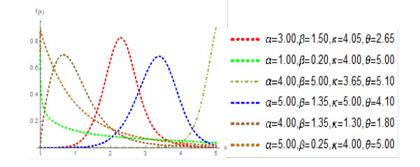
We propose a new four-parameter lifetime model with flexible hazard rate called the Burr XII Power Cauchy (BXII-PC) distribution. We derive the BXII-PC distribution via (ⅰ) the T-X family technique and (ⅱ) nexus between the exponential and gamma variables. The new proposed distribution is flexible as it has famous sub-models such as Burr XII-half Cauchy, Lomax-power Cauchy, Lomax-half Cauchy, Log-logistic-power Cauchy, log-logistic-half Cauchy. The failure rate function for the BXII-PC distribution is flexible as it can accommodate various shapes such as the modified bathtub, inverted bathtub, increasing, decreasing; increasing-decreasing and decreasing-increasing-decreasing. Its density function can take shapes such as exponential, J, reverse-J, left-skewed, right-skewed and symmetrical. To illustrate the importance of the BXII-PC distribution, we establish various mathematical properties such as random number generator, moments, inequality measures, reliability measures and characterization. Six estimation methods are used to estimate the unknown parameters of the proposed distribution. We perform a simulation study on the basis of the graphical results to demonstrate the performance of the maximum likelihood, maximum product spacings, least squares, weighted least squares, Cramer-von Mises and Anderson-Darling estimators of the parameters of the BXII-PC distribution. We consider an application to a real data set to prove empirically the potentiality of the proposed model.

| [1] |
P. R. Rider, Generalized Cauchy distribution, Ann. Math. Stat., 9 (1957), 215-223. doi: 10.1007/BF02892507

|
| [2] |
R. C. Dahiya, P. G. Staneski, N. R. Chaganty, Maximum likelihood estimation of parameters of the truncated Cauchy distribution, Commun. Stat. Theory Methods, 30 (2001), 1737-1750. doi: 10.1081/STA-100105695
|
| [3] |
S. Nadarajah, S. Kotz, A truncated Cauchy distribution, Int. J. Math. Educ. Sci. Technol., 37 (2006), 605-608. doi: 10.1080/00207390600595223
|
| [4] | N. L. Johnson, S. Kotz, N. Balakrishnan, Continuous Univariate Distributions, Second edition, New York: Wiley, 1994. |
| [5] |
N. Eugene, C. Lee, F. Famoye, Beta-normal distribution and its applications, Commun. Stat. Theory Methods, 31 (2002), 497-512. doi: 10.1081/STA-120003130
|
| [6] | E. Alshawarbeh, F. Famoye, C. Lee, Beta-Cauchy distribution: Some properties and applications, J. Stat. Theory Appl., 12 (2013), 378-391. |
| [7] | E. Alshawarbeh, C. Lee, F. Famoye, The beta-Cauchy distribution, J. Probab. Stat. Sci., 10 (2012), 41-57. |
| [8] | E. Jacob, K. Jayakumar, On half-Cauchy distribution and process, Int. J. Stat. Math., 3 (2012), 77-81. |
| [9] | G. M. Cordeiro, A. J. Lemonte, The beta-half Cauchy distribution, J. Probab. Stat., 2011 (2011), 904705. |
| [10] | G. G. Hamedani, I. Ghosh, Kumaraswamy-half-Cauchy distribution: Characterizations and related results, Int. J. Stat. Probab., 4 (2015), 94-100. |
| [11] | M. H. Tahir, M. Zubair, G. M. Cordeiro, A. Alzaatreh, M. Mansoor, The Weibull-Power Cauchy distribution: Model, properties and applications, Hacettepe J. Math. Stat., 46 (2017), 767-789. |
| [12] | J. E. Contreras-Reyes, F. Kahrari, D. D. Cortés, On the modified skew-normal-Cauchy distribution: Properties, inference and applications, Commun. Stat. Theory Methods, (2020), 1-17. |
| [13] |
I. W. Burr, Cumulative frequency functions, Ann. Math. Stat., 13 (1942), 215-232. doi: 10.1214/aoms/1177731607
|
| [14] | R. B. Silva, G. M. Cordeiro, The Burr XII power series distributions: A new compounding family, Braz. J. Probab. Stat., 29 (2015), 565-589. |
| [15] |
I. Elbatal, E. Altun, A. Z. Afify, G. Ozel, The generalized Burr XII power series distributions with properties and applications, Ann. Data Sci., 6 (2019), 571-597. doi: 10.1007/s40745-018-0171-2
|
| [16] |
G. M. Cordeiro, H. M. Yousof, T. G. Ramires, E. M. Ortega, The Burr XII system of densities: Properties, regression model and applications, J. Stat. Comput. Simul., 88 (2018), 432-456. doi: 10.1080/00949655.2017.1392524
|
| [17] |
H. Goual, H. M. Yousof, Validation of Burr XII inverse Rayleigh model via a modified chi-squared goodness-of-fit test, J. Appl. Stat., 47 (2020), 393-423. doi: 10.1080/02664763.2019.1639642
|
| [18] |
F. A. Bhatti, G. G. Hamedani, M. Ç. Korkmaz, W. Sheng, A. Ali, On the Burr XII-moment exponential distribution, Plos One, 16 (2021), e0246935. doi: 10.1371/journal.pone.0246935
|
| [19] | A. Alzaatreh, M. Mansoor, M. H. Tahir, M. Zubair, S. Ali, The gamma half-Cauchy distribution: Properties and applications, Hacettepe J. Math. Stat., 45 (2016), 1143-1159. |
| [20] | B. Rooks, A. Schumacher, K. Cooray, The power Cauchy distribution: Derivation, description, and composite models, NSF-REU Program Reports, 2010. |
| [21] | M. H. Tahir, M. Zubair, G. M. Cordeiro, A. Alzaatreh, M. Mansoor, The Weibull-Power Cauchy distribution: Model, properties and applications, Hacettepe J. Math. Stat., 46 (2017), 767-789. |
| [22] |
G. K. Bhattacharyya, R. A. Johnson, Estimation of reliability in a multicomponent stress-strength model, J. Am. Stat. Assoc., 69 (1974), 966-970. doi: 10.1080/01621459.1974.10480238
|
| [23] |
S. Kotz, C. D. Lai, M. Xie, On the effect of redundancy for systems with dependent components, IIE Trans, 35 (2003), 1103-1110. doi: 10.1080/714044440
|
| [24] | W. Glänzel, A characterization theorem based on truncated moments and its application to some distribution families, In: P. Bauer, F. Konecny, W. Wertz, Mathematical Statistics and Probability Theory, Dordrecht: Springer, 1987. |
| [25] |
W. Glänzel, Some consequences of a characterization theorem based on truncated moments, Statistics, 21 (1990), 613-618. doi: 10.1080/02331889008802273
|
| [26] | R. C. H. Cheng, N. A. K. Amin, Maximum product of spacings estimation with application to the lognormal distribution, Math. Report, (1979), 791. |
| [27] | R. C. H. Cheng, N. A. K. Amin, Estimating parameters in continuous univariate distributions with a shifted origin, J. R. Stat. Soc. Ser. B, 45 (1983), 394-403. |
| [28] | B. Ranneby, The maximum spacing method. An estimation method related to the maximum likelihood method, Scand. J. Stat., 11 (1984), 93-112. |
| [29] |
T. W. Anderson, D. A. Darling, Asymptotic theory of certain "goodness of fit" criteria based on stochastic processes, Ann. Math. Stat., 23 (1952), 193-212. doi: 10.1214/aoms/1177729437
|
| [30] |
G. Chen, N. Balakrishnan, A general purpose approximate goodness-of-fit test, J. Qual. Technol., 27 (1995), 154-161. doi: 10.1080/00224065.1995.11979578
|
| [31] |
F. Proschan, Theoretical explanation of observed decreasing failure rate, Technometrics, 5 (1963), 375-383. doi: 10.1080/00401706.1963.10490105
|


Figures(7) / Tables(3)

Fiaz Ahmad Bhatti, G. G. Hamedani, Mashail M. Al Sobhi, Mustafa Ç. Korkmaz. On the Burr XII-Power Cauchy distribution: Properties and applications[J]. AIMS Mathematics, 2021, 6(7): 7070-7092. doi: 10.3934/math.2021415


 DownLoad: