A novel asymmetric form of the power half-logistic distribution with statistical inference and real data analysis

Amal S. Hassan; Najwan Alsadat; Mohammed Elgarhy; Laxmi Prasad Sapkota; Oluwafemi Samson Balogun; Ahmed M. Gemeay; Amal S. Hassan; Najwan Alsadat; Mohammed Elgarhy; Laxmi Prasad Sapkota; Oluwafemi Samson Balogun; Ahmed M. Gemeay

doi:10.3934/era.2025036

Electronic Research Archive

2025, Volume 33, Issue 2: 791-825. doi: 10.3934/era.2025036

Previous Article Next Article

Research article

A novel asymmetric form of the power half-logistic distribution with statistical inference and real data analysis

1.
Faculty of Graduate Studies for Statistical Research, Cairo University, 5 Dr. Ahmed Zewail Street, Giza 12613, Egypt
2.
Department of Quantitative Analysis, College of Business Administration, King Saud University, P.O. Box 71115, Riyadh 11587, Saudi Arabia
3.
Department of Basic Sciences, Higher Institute of Administrative Sciences, Belbeis, AlSharkia, Egypt
4.
Department of Statistics, Tribhuvan University, Tribhuvan Multiple Campus, Palpa, Nepal
5.
Department of Computing, University of Eastern Finland, FI-70211, Finland
6.
Department of Mathematics, Faculty of Science, Tanta University, Tanta 31527, Egypt

Received: 09 July 2024 Revised: 30 December 2024 Accepted: 08 January 2025 Published: 12 February 2025

This study provided a significant contribution to developing an adaptable trigonometric extension of the power half-logistic distribution. To be more specific, we created an innovative two-parameter lifetime model called the sine power half-logistic distribution (SPHLD) by using features from the sine-generated family of distributions. The novel distribution could be more effective in modeling lifetime phenomena when asymmetric data was presented, which was the primary motivating factor. The SPHLD's density function plots showed that the distribution adopted several asymmetric shape configurations. Furthermore, the SPHLD's hazard rate plots displayed both monotonic increases and decreases. The quantile function, moments, incomplete moment, and stress-strength reliability were among the statistical characteristics of the SPHLD that were computed. Statistical inference using sixteen distinct classical estimating techniques was utilized to estimate the SPHLD parameters. A simulation study was done to evaluate the consistency of the different estimates and determine the best estimating approach based on some accuracy measures. Analyses of real data revealed that the SPHLD performed better than a number of alternative distributions.
Citation: Amal S. Hassan, Najwan Alsadat, Mohammed Elgarhy, Laxmi Prasad Sapkota, Oluwafemi Samson Balogun, Ahmed M. Gemeay. A novel asymmetric form of the power half-logistic distribution with statistical inference and real data analysis[J]. Electronic Research Archive, 2025, 33(2): 791-825. doi: 10.3934/era.2025036

Related Papers:

Abstract

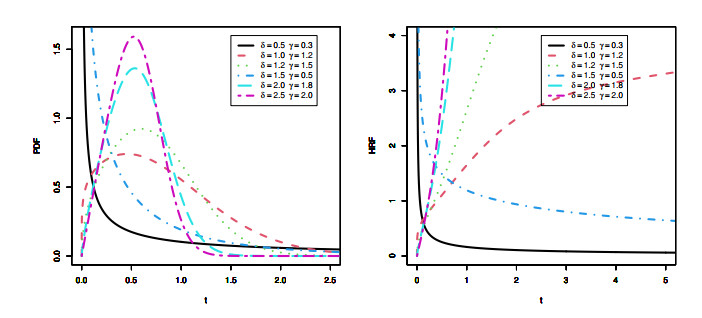
This study provided a significant contribution to developing an adaptable trigonometric extension of the power half-logistic distribution. To be more specific, we created an innovative two-parameter lifetime model called the sine power half-logistic distribution (SPHLD) by using features from the sine-generated family of distributions. The novel distribution could be more effective in modeling lifetime phenomena when asymmetric data was presented, which was the primary motivating factor. The SPHLD's density function plots showed that the distribution adopted several asymmetric shape configurations. Furthermore, the SPHLD's hazard rate plots displayed both monotonic increases and decreases. The quantile function, moments, incomplete moment, and stress-strength reliability were among the statistical characteristics of the SPHLD that were computed. Statistical inference using sixteen distinct classical estimating techniques was utilized to estimate the SPHLD parameters. A simulation study was done to evaluate the consistency of the different estimates and determine the best estimating approach based on some accuracy measures. Analyses of real data revealed that the SPHLD performed better than a number of alternative distributions.

References

[1]	A. Marshall, I. Olkin, A new method for adding a parameter to a family of distributions with applications to the exponential and Weibull families, Biometrika, 84 (1997), 641–652. https://doi.org/10.1093/biomet/84.3.641 doi: 10.1093/biomet/84.3.641
[2]	N. Eugene, C. Lee, F. Famoye, Beta-normal distribution and its applications, Commun. Stat.-Theory Methods, 31 (2002), 497–512. https://doi.org/10.1081/STA-120003130 doi: 10.1081/STA-120003130
[3]	A. Alzaatreh, F. Famoye, C. Lee, A new method for generating families of continuous distributions, Metron, 71 (2013), 63–79. https://doi.org/10.1007/s40300-013-0007-y doi: 10.1007/s40300-013-0007-y
[4]	A. Al-Shomrani, O. Arif, A. Shawky, S. Hanif, M. Q. Shahbaz, Topp-Leone family of distributions: Some properties and application, Pak. J. Stat. Oper. Res., 12 (2016), 443–451. https://doi.org/10.18187/pjsor.v12i3.1458 doi: 10.18187/pjsor.v12i3.1458
[5]	A. S. Hassan, E. A. El-Sherpieny, S. A. El-Taweel, New Topp Leone-G family with mathematical properties and applications, J. Phys.: Conf. Ser., 12 (2021). https://doi:10.1088/1742-6596/1860/1/012011. doi: 10.1088/1742-6596/1860/1/012011
[6]	M. A. Badr, I. Elbatal, F. Jamal, C. Chesneau, M. Elgarhy, The transmuted odd Fréchet-G family of distributions: Theory and applications, Mathematics, 8 (2020), 958. https://doi.org/10.3390/math8060958 doi: 10.3390/math8060958
[7]	M. Aslam, Z. Asghar, Z. Hussain, S. F. Shah, A modified T-X family of distributions: Classical and Bayesian analysis, J. Taibah Univ. Sci., 14 (2020), 254–264. https://doi.org/10.1080/16583655.2020.1732642 doi: 10.1080/16583655.2020.1732642
[8]	A. S. Hassan, M. A. H. Sabry, A. M. Elsehtery, A new probability distribution family arising from truncated power Lomax distribution with application to Weibull model, Pak. J. Stat. Oper. Res., 16 (2020), 661–674. https://doi.org/10.1007/s12015-020-09979-4 doi: 10.1007/s12015-020-09979-4
[9]	F. S. Gomes-Silva, A. Percontini, E. de Brito, M. W. Ramos, R. Venâncio, G. M. Cordeiro, The odd Lindley-G family of distributions, Austrian J. Stat., 46 (2017), 65–87. https://doi.org/10.17713/ajs.v46i1.222 doi: 10.17713/ajs.v46i1.222
[10]	A. S. Hassan, S. G. Nassar, Power Lindley-G family of distributions, Ann. Data Sci., 6 (2019), 189–210. https://doi.org/10.1007/s40745-018-0159-y doi: 10.1007/s40745-018-0159-y
[11]	I. Elbatal, N. Alotaibi, E. M. Almetwally, S. A. Alyami, M. Elgarhy, On odd perks-G class of distributions: properties, regression model, discretization, Bayesian and non-Bayesian estimation, and applications, Symmetry, 14 (2022), 883. https://doi.org/10.3390/sym14050883 doi: 10.3390/sym14050883
[12]	A. Z. Afify, G. M. Cordeiro, N. A. Ibrahim, J. M. Elgarhy, M. A. Nasir, The Marshall-Olkin odd Burr Ⅲ-G family: Theory, estimation, and engineering applications, IEEE Access, 9 (2021), 4376–4387. https://doi.org/10.1109/ACCESS.2020.3044156 doi: 10.1109/ACCESS.2020.3044156
[13]	C. Chesneau, T. E. Achi, Modified odd Weibull family of distributions: Properties and applications, J. Indian Soc. Probab. Stat., 21 (2020), 259–286. https://doi.org/10.1007/s41096-020-00075-x doi: 10.1007/s41096-020-00075-x
[14]	J. T. Eghwerido, D. J. Ikwuoche, O. D. AdubisiM, Inverse odd Weibull generated family of distribution, Pak. J. Stat. Oper. Res., 16 (2020), 617—633.
[15]	D. Kumar, U. Singh, S. K. Singh, A new distribution using sine function- its application to bladder cancer patients data, J. Stat. Appl. Prob., 4 (2015), 417–427.
[16]	Z. Mahmood, C. Chesneau, M.H. Tahir, A new sine-G family of distributions: properties and applications, Bull. Comput. Appl. Math., 7 (2019), 53–81.
[17]	N. Balakrishnan, Order statistics from the half logistic distribution. J. Stat. Comput. Simul., 20 (1985), 287–309.
[18]	R. S. Rao, P. L. Mamidi, R. R. Kantam, Modified maximum likelihood estimation: Inverse half logistic distribution, J. Math., 5 (2016), 11–19.
[19]	H. Torabi, F. L. Bagheri, Estimation of parameters for an extended generalized half logistic distribution based on complete and censored data, J. Iranian Stat. Soc., 9 (2010), 171–195.
[20]	G. M. Cordeiro, M. Alizadeh, E. M. M. Ortega, The exponentiated half logistic family of distributions: properties and applications, J. Probab. Stat., 2014 (2014), 864396. https://doi.org/10.1155/2014/864396 doi: 10.1155/2014/864396
[21]	J. Oliveira, J. Santos, C. Xavier, D. Trindade, G. M. Cordeiro, The McDonald half-logistic distribution: theory and practice, Commun. Stat. Theory Methods, 45 (2016), 2005–2022. https://doi.org/10.1080/03610926.2013.873131 doi: 10.1080/03610926.2013.873131
[22]	A. H. Hassan, M. Elgarhy, M. Shakil, Type Ⅱ half logistic family of distributions with applications, Pak. J. Stat. Oper. Res., 13 (2017), 245–264. https://doi.org/10.18187/pjsor.v13i2.1560 doi: 10.18187/pjsor.v13i2.1560
[23]	S. D. Krishnarani, On a power transformation of half-logistic distribution, J. Probab. Stat., 20 (2016), 1–10.
[24]	R. M. Usman, A. M. Haq, J. Talib, Kumaraswamy half-logistic distribution: properties and applications, J. Stat. Appl. Probab., 6 (2017), 597–609. https://doi.org/10.18576/jsap/060315 doi: 10.18576/jsap/060315
[25]	D. Yegen, G. Ozel, Marshall-Olkin half logistic distribution with theory and applications, Alphanum. J., 6 (2018), 408–416. https://doi.org/10.17093/alphanumeric.409992 doi: 10.17093/alphanumeric.409992
[26]	M. Elgarhy, A. S. Hassan, S. Fayomi, Maximum likelihood and Bayesian estimation for two-parameter type Ⅰ half logistic Lindley distribution, J. Comput. Theor. Nanosci., 15 (2018), 1–9. https://doi.org/10.1166/jctn.2018.7600 doi: 10.1166/jctn.2018.7600
[27]	A. F. Samuel, O. A. Kehinde, A study on transmuted half logistic distribution: Properties and application, Int. J. Stat. Distribut. Appl., 5 (2019), 54–59.
[28]	A. S. Hassan, M. Elgarhy, M. A. Haq, S. Alrajhi, On type Ⅱ half logistic Weibull distribution with applications, Math. Theory Model., 19(2019), 49–63. https://doi.org/10.21608/esju.2019.268726 doi: 10.21608/esju.2019.268726
[29]	M. Anwar, A. Bibi, The half-logistic generalized Weibull distribution, J. Probab. Stat., (2018), 8767826. https://doi.org/10.1155/2018/8767826 doi: 10.1155/2018/8767826
[30]	A. Algarni, A. M. Almarashi, I. Elbatal, A. S. Hassan, E. M. Almetwally, c Daghistani, et al., Type Ⅰ half logistic Burr X-G family: Properties, Bayesian, and non-Bayesian estimation under censored samples and applications to COVID-19 data, Math. Probl. Eng., 2021, (2021), 5461130. https://doi.org/10.1155/2021/5461130 doi: 10.1155/2021/5461130
[31]	G. S. Mohammad, A new two-parameter modified half-logistic distribution: Properties and Applications, Stat. Optim. Inf. Comput., 10 (2022), 589–605. https://doi.org/10.19139/soic-2310-5070-1210 doi: 10.19139/soic-2310-5070-1210
[32]	A. S. Hassan, A. Fayomi, A. Algarni, E. M. Almetwally, Bayesian and non-Bayesian inference for unit-exponentiated half-logistic distribution with data analysis, Appl. Sci., 12 (2022), 11253. https://doi.org/10.3390/app122111253 doi: 10.3390/app122111253
[33]	H. Majid, An extended type Ⅰ half-logistic family of distributions: Properties, applications and different method of estimations, Math. Slovaca, 72 (2022), 745–764. https://doi.org/10.1515/ms-2022-0051 doi: 10.1515/ms-2022-0051
[34]	R. M. I. Arshad, M. H. Tahir, C. Chesneau, S. Khan, F. Jamal, The gamma power half-logistic distribution: theory and applications, Sao Paulo J. Math. Sci., 17 (2023), 1142–1169. https://doi.org/10.1007/s40863-022-00331-x doi: 10.1007/s40863-022-00331-x
[35]	S. M. Alghamdi, M. Shrahili, A. S. Hassan, A. M. Gemeay, I. Elbatal, M. Elgarhy, Statistical inference of the half logistic modified Kies exponential model with modeling to engineering data, Symmetry, 15 (2023), 586. https://doi.org/10.3390/sym15030586 doi: 10.3390/sym15030586
[36]	O. D. Adubisi, C. E. Adubisi, Novel distribution for modeling uncensored and censored survival time data and regression model, Reliab. Theory Appl., 3 (2023), 808–824.
[37]	R. C. H. Cheng, N. A. K. Amin, Maximum product-of-spacings estimation with applications to the log-normal distribution, University of Wales IST, Math Report, (1979), 79–103.
[38]	R. C. H. Cheng, N. A. K. Amin, Estimating parameters in continuous univariate distributions with a shifted origin, J. R. Stat. Soc.: Ser. B (Methodol.) 45 (1983), 394–403. https://doi.org/10.1111/j.2517-6161.1983.tb01268.x
[39]	B. Ranneby, The maximum spacing method: An estimation method related to the maximum likelihood method, Scand. J. Stat., 11 (1984), 93–112.
[40]	G. M. Cordeiro, T. A. de Andrade, M. Bourguignon, F. G. Silva, The exponentiated generalized standardized half-logistic distribution, Int. J. Stat. Probab., 6 (2017), 24–42. https://doi.org/10.5539/ijsp.v6n3p24 doi: 10.5539/ijsp.v6n3p24
[41]	J. I. Seo, S. B. Kang, Notes on the exponentiated half logistic distribution, Appl. Math. Model., 39 (2015), 6491–6500.
[42]	M. Muhammad, L. Liu, A new extension of the generalized half logistic distribution with applications to real data, Entropy, 21 (2019), 339. https://doi.org/10.3390/e21040339 doi: 10.3390/e21040339
[43]	R. M. Usman, M. Haq, J. Talib, Kumaraswamy half-logistic distribution: properties and applications, J. Stat. Appl. Probab., 6 (2017), 597–609. https://doi.org/10.18576/jsap/060315 doi: 10.18576/jsap/060315
[44]	G. M. Cordeiro, R. B. dos Santos, The beta power distribution. Brazil J. Probab. Stat., 26 (2012), 88–112. https://doi.org/10.1214/10-BJPS124 doi: 10.1214/10-BJPS124
[45]	M. V. Aarset, How to identify a bathtub hazard rate, IEEE Trans. Reliab., 36 (1987), 106–108. https://doi.org/10.1109/TR.1987.5222310 doi: 10.1109/TR.1987.5222310
[46]	E. T. Lee, Statistical methods for survival data analysis, IEEE Trans. Reliab., 35 (1986), 123–123. https://doi.org/10.1109/TR.1986.4335370 doi: 10.1109/TR.1986.4335370
[47]	A. Henningsen, O. Toomet, maxLik: A package for maximum likelihood estimation in R, Comput. Stat., 26 (2011), 443–458. https://doi.org/10.1007/s00180-010-0217-1 doi: 10.1007/s00180-010-0217-1
[48]	R Core Team, R: A language and environment for statistical computing, Foundation for Statistical Computing, Vienna, Austria, 2013.
[49]	B. Lambert, A student's guide to Bayesian statistics, in A Student's Guide to Bayesian Statistics, (2018), 1–520.
[50]	K. P. Burnham, D. R. Anderson, Model selection and multimodel inference: a practical information-theoretic approach, Springer, 2002.

Reader Comments

Your name:*

Email:*
© 2025 the Author(s), licensee AIMS Press. This is an open access article distributed under the terms of the Creative Commons Attribution License (http://creativecommons.org/licenses/by/4.0)