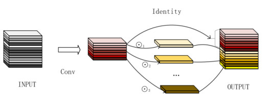
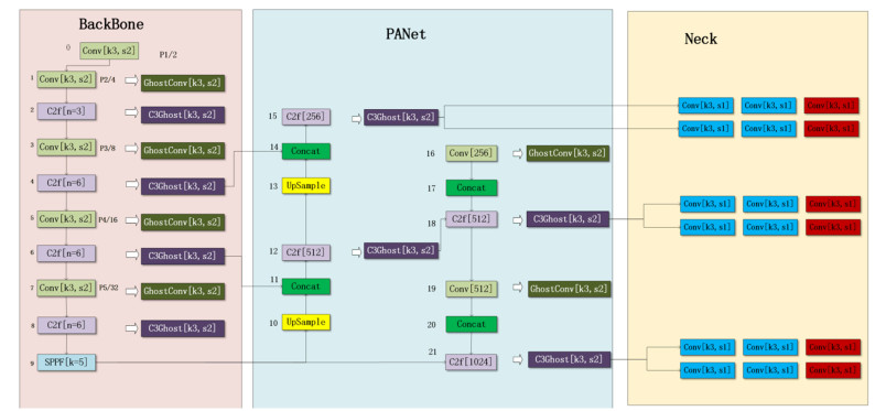
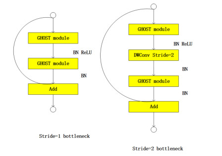
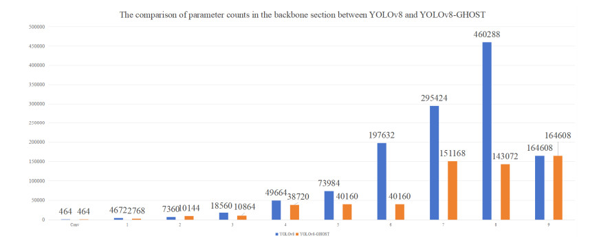
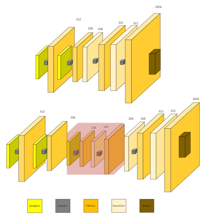
Breast cancer has a very high incidence rate worldwide, and effective screening and early diagnosis are particularly important. In this paper, two improved You Only Look Once version 8 (YOLOv8) models, the YOLOv8-GHOST and YOLOv8-P2 models, are proposed to address the difficulty of distinguishing lesions from normal tissues in mammography images. The YOLOv8-GHOST model incorporates GHOSTConv and C3GHOST modules into the original YOLOv8 model to capture richer feature information while using only 57% of the number of parameters required by the original model. The YOLOv8-P2 algorithm significantly reduces the number of necessary parameters by streamlining the number of channels in the feature map. This paper proposes the YOLOv8-GHOST-P2 model by combining the above two improvements. Experiments conducted on the MIAS and DDSM datasets show that the new models achieved significantly improved computational efficiency while maintaining high detection accuracy. Compared with the traditional YOLOv8 method, the three new models improved and achieved F1 scores of 98.38%, 98.8%, and 98.57%, while the number of parameters reduced by 42.9%, 46.64%, and 2.8%. These improvements provide a more efficient and accurate tool for clinical breast cancer screening and lay the foundation for subsequent studies. Future work will explore the potential applications of the developed models to other medical image analysis tasks.
Citation: Yihua Lan, Yingjie Lv, Jiashu Xu, Yingqi Zhang, Yanhong Zhang. Breast mass lesion area detection method based on an improved YOLOv8 model[J]. Electronic Research Archive, 2024, 32(10): 5846-5867. doi: 10.3934/era.2024270
Breast cancer has a very high incidence rate worldwide, and effective screening and early diagnosis are particularly important. In this paper, two improved You Only Look Once version 8 (YOLOv8) models, the YOLOv8-GHOST and YOLOv8-P2 models, are proposed to address the difficulty of distinguishing lesions from normal tissues in mammography images. The YOLOv8-GHOST model incorporates GHOSTConv and C3GHOST modules into the original YOLOv8 model to capture richer feature information while using only 57% of the number of parameters required by the original model. The YOLOv8-P2 algorithm significantly reduces the number of necessary parameters by streamlining the number of channels in the feature map. This paper proposes the YOLOv8-GHOST-P2 model by combining the above two improvements. Experiments conducted on the MIAS and DDSM datasets show that the new models achieved significantly improved computational efficiency while maintaining high detection accuracy. Compared with the traditional YOLOv8 method, the three new models improved and achieved F1 scores of 98.38%, 98.8%, and 98.57%, while the number of parameters reduced by 42.9%, 46.64%, and 2.8%. These improvements provide a more efficient and accurate tool for clinical breast cancer screening and lay the foundation for subsequent studies. Future work will explore the potential applications of the developed models to other medical image analysis tasks.

| [1] |
X. Pei, R. Zhou, Current status and future of Chinese medicine diagnosis and treatment of breast cancer (in Chinese), Beijing Tradit. Chin. Med., 42 (2023), 704–707. https://doi.org/10.16025/j.1674-1307.2023.07.001 doi: 10.16025/j.1674-1307.2023.07.001

|
| [2] | E. Mahoro, M. A. Akhloufi, Breast masses detection on mammograms using recent one-shot deep object detectors, in 2023 5th International Conference on Bio-engineering for Smart Technologies (BioSMART), IEEE, (2023), 1–4. https://doi.org/10.1109/BioSMART58455.2023.10162036 |
| [3] | A. Intasam, Y. Promworn, A. Juhong, S. Thanasitthichai, S. Khwayotha, T. Jiranantanakorn, et al., Optimizing the hyperparameter tuning of yolov5 for breast cancer detection, in 2023 9th International Conference on Engineering, Applied Sciences, and Technology (ICEAST), IEEE, (2023), 184–187. https://doi.org/10.1109/ICEAST58324.2023.10157611 |
| [4] | X. Gao, B. Braden, S. Taylor, W. Pang, Towards real-time detection of squamous pre-cancers from oesophageal endoscopic videos, in 2019 18th IEEE International Conference On Machine Learning And Applications (ICMLA), IEEE, (2019), 1606–1612. https://doi.org/10.1109/ICMLA.2019.00264 |
| [5] |
Y. Yang, J. Wang, Research on breast cancer pathological image classification method based on wavelet transform and YOLOv8, J. X-Ray Sci. Technol., 32 (2024), 677–687. https://doi.org/10.3233/XST-230296 doi: 10.3233/XST-230296
|
| [6] |
M. A. Al-Antari, S. Han, T. Kim, Evaluation of deep learning detection and classification towards computer-aided diagnosis of breast lesions in digital X-ray mammograms, Comput. Methods Programs Biomed., 196 (2020), 105584. https://doi.org/10.1016/j.cmpb.2020.105584 doi: 10.1016/j.cmpb.2020.105584
|
| [7] | M. A. Al-masni, M. A. Al-antari, J. M. Park, G. Gi, T. Y. Kim, P. Rivera, et al., Detection and classification of the breast abnormalities in digital mammograms via regional convolutional neural network, in 2017 39th Annual International Conference of the IEEE Engineering in Medicine and Biology Society (EMBC), IEEE, (2017), 1230–1233. https://doi.org/10.1109/EMBC.2017.8037053 |
| [8] | R. K. Kassahun, M. Molinara, A. Bria, C. Marrocco, F Tortorella, Breast mass detection and classification using transfer learning on OPTIMAM dataset through RadImageNet weights, in International Conference on Image Analysis and Processing, Springer, (2024), 71–82. https://doi.org/10.1007/978-3-031-51026-7_7 |
| [9] | F. Touazi, D. Gaceb, M. Chirane, S. Hrzallah, Two-stage approach for semantic image segmentation of breast cancer: Deep learning and mass detection in mammographic images, in 6th International Workshop on Informatics & Data-Driven Medicine (IDDM), CEUR Workshop Proceedings, (2023), 62–76. https://doi.org/10.1109/iciprob54042.2022.9798724 |
| [10] | W. Ouyang, P. Luo, X. Zeng, S. Qiu, Y. Tian, H. Li, et al., Deepid-net: Multi-stage and deformable deep convolutional neural networks for object detection, preprint, arXiv: 1409.3505. |
| [11] | C. Szegedy, W. Liu, Y. Jia, P. Sermanet, S. Reed, D. Anguelov, et al., Going deeper with convolutions, in 2015 IEEE Conference on Computer Vision and Pattern Recognition (CVPR), IEEE, (2015), 1–9. https://doi.org/10.1109/CVPR.2015.7298594 |
| [12] | S. Cheng, G. Shang, L. Zhang, Handwritten digit recognition based on improved VGG16 network, in Tenth International Conference on Graphics and Image Processing (ICGIP 2018), (2019), 110693B. https://doi.org/10.1117/12.2524281 |
| [13] | B. Zoph, Q. V. Le, Neural architecture search with reinforcement learning, preprint, arXiv: 1611.01578. |
| [14] | D. Cai, X. Sun, N. Zhou, X. Han, J. Yao, Efficient mitosis detection in breast cancer histology images by RCNN, in 2019 IEEE 16th International Symposium on Biomedical Imaging (ISBI 2019), IEEE, (2019), 919–922. https://doi.org/10.1109/ISBI.2019.8759461 |
| [15] |
S. Ren, K. He, R. Girshick, J. Sun, Faster R-CNN: Towards real-time object detection with region proposal networks, IEEE Trans. Pattern Anal. Mach. Intell., 39 (2016), 1137–1149. https://doi.org/10.1109/TPAMI.2016.2577031 doi: 10.1109/TPAMI.2016.2577031
|
| [16] |
T. Mahmood, M. Arsalan, M. Owais, M. B. Lee, K. R. Park, Artificial intelligence-based mitosis detection in breast cancer histopathology images using faster R-CNN and deep CNNs, J. Clin. Med., 9 (2020), 749. https://doi.org/10.3390/jcm9030749 doi: 10.3390/jcm9030749
|
| [17] | J. Redmon, S. Divvala, R. Girshick, A. Farhadi, You only look once: Unified, real-time object detection, preprint, arXiv: 1506.02640. |
| [18] | S. R. Sindhu, J. George, S. Skaria, V. V. Varun, Using YOLO based deep learning network for real time detection and localization of lung nodules from low dose CT scans, in Medical Imaging 2018: Computer-Aided Diagnosis, SPIE, 10575 (2018), 347–355. https://doi.org/10.1117/12.2293699 |
| [19] |
H. M. Ünver, E. Ayan, Skin lesion segmentation in dermoscopic images with combination of YOLO and grabcut algorithm, Diagnostics, 9 (2019), 72. https://doi.org/10.3390/diagnostics9030072 doi: 10.3390/diagnostics9030072
|
| [20] | J. Sobek, J. R. M. Inojosa, B. J. M. Inojosa, S. M. Rassoulinejad-Mousavi, G, M. Conte, F. Lopez-Jimenez, et al., MedYOLO: A medical image object detection framework, J. Digit. Imaging. Inform. Med., (2024), 1–9. https://doi.org/10.1007/s10278-024-01138-2 |
| [21] | K. Han, Y. Wang, Q. Tian, J. Guo, C. Xu, C. Xu, Ghostnet: More features from cheap operations, in 2020 IEEE/CVF Conference on Computer Vision and Pattern Recognition (CVPR), IEEE, (2020), 1577–1586. https://doi.org/10.1109/CVPR42600.2020.00165 |
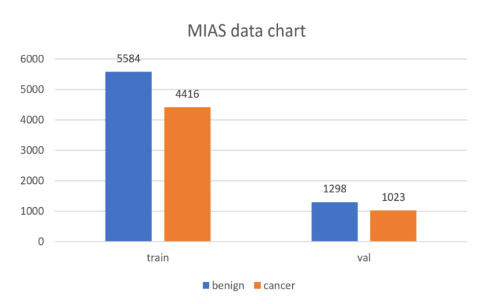
| [22] | J. Suckling, J. Parker, D. Dance, S. Astley, I. Hutt, C. Boggis, et al., Mammographic Image Analysis Society (MIAS) database v1.21, Apollo-University of Cambridge Repository, 2015. https://doi.org/10.17863/CAM.105113 |
| [23] |
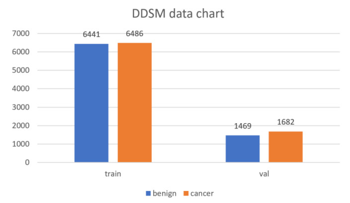
M. Heath, K. Bowyer, D. Kopans, P. K. Jr, R. Moore, K. Chang, et al., Current status of the digital database for screening mammography, Digital Mammography, 13 (1998), 457–460. https://doi.org/10.1007/978-94-011-5318-8_75 doi: 10.1007/978-94-011-5318-8_75
|
Figures(9) / Tables(8)
Yihua Lan, Yingjie Lv, Jiashu Xu, Yingqi Zhang, Yanhong Zhang. Breast mass lesion area detection method based on an improved YOLOv8 model[J]. Electronic Research Archive, 2024, 32(10): 5846-5867. doi: 10.3934/era.2024270


 DownLoad: