A stochastic model of leptospirosis with vector and environmental transmission is established in this paper. By mathematical analysis of the model, the threshold for eliminating the disease is obtained. The partial rank correlation coefficient was used to analyze the parameters that have a greater impact on disease elimination, and a sensitivity analysis was conducted on the parameters through numerical simulation. Further, combined with the data of leptospirosis case reports in China from 2003 to 2021, two parameter estimation methods, Least Squares method (LSM) and Markov Chain Monte Carlo-Metropolis Hastings method (MCMC-MH), are applied to estimate the important parameters of the model and the future trend of leptospirosis in China are predicted.
Citation: Xiangyun Shi, Dan Zhou, Xueyong Zhou, Fan Yu. Predicting the trend of leptospirosis in China via a stochastic model with vector and environmental transmission[J]. Electronic Research Archive, 2024, 32(6): 3937-3951. doi: 10.3934/era.2024176
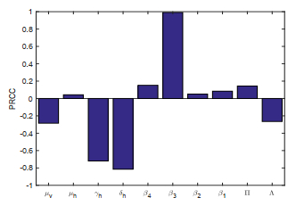
A stochastic model of leptospirosis with vector and environmental transmission is established in this paper. By mathematical analysis of the model, the threshold for eliminating the disease is obtained. The partial rank correlation coefficient was used to analyze the parameters that have a greater impact on disease elimination, and a sensitivity analysis was conducted on the parameters through numerical simulation. Further, combined with the data of leptospirosis case reports in China from 2003 to 2021, two parameter estimation methods, Least Squares method (LSM) and Markov Chain Monte Carlo-Metropolis Hastings method (MCMC-MH), are applied to estimate the important parameters of the model and the future trend of leptospirosis in China are predicted.

| [1] | L. Liu, H. Zhu, G. Yang, Current situation of endemic status, prevention and control of neglected zoonotic diseases in China (in Chinese), Chin. J. Schistosomiasis Control, 25 (2013), 307–311. |
| [2] |
H. T. Alemneh, A co-infection model of dengue and leptospirosis diseases, Adv. Differ. Equations, 2020 (2020), 664–687. https://doi.org/10.1186/s13662-020-03126-6 doi: 10.1186/s13662-020-03126-6

|
| [3] | A. Bhalraj, A. Azmi, M. H. Mohd, Analytical and numerical solutions of leptospirosis model, Comput. Sci., 16 (2021), 949–961. |
| [4] |
M. A. Gallego, M. V. Simoy, Mathematical modeling of leptospirosis: a dynamic regulated by environmental carrying capacity, Chaos, Solitons Fractals, 152 (2021), 111425. https://doi.org/10.1016/j.chaos.2021.111425 doi: 10.1016/j.chaos.2021.111425
|
| [5] |
H. A. Engida, D. M. Theuri, D. Gathungu, J. Gachohi, H. T. Alemneh, A mathematical model analysis for the transmission dynamics of leptospirosis disease in human and rodent populations, Comput. Math. Methods Med., 2022 (2022), 1806585. https://doi.org/10.1155/2022/1806585 doi: 10.1155/2022/1806585
|
| [6] |
D. Baca-Carrasco, D. Olmos, I. Barradas, A mathematical model for human and animal leptospirosis, J. Biol. Syst., 23 (2015), S55–S65. https://doi.org/10.1142/S0218339015400057 doi: 10.1142/S0218339015400057
|
| [7] |
D. Zhou, X. Y. Shi, X. Y. Zhou, Dynamic analysis of a stochastic delayed SEIRS epidemic model with Lévy jumps and the impact of public health education, Axioms, 12 (2023), 560. https://doi.org/10.3390/axioms12060560 doi: 10.3390/axioms12060560
|
| [8] |
J. Djordjevic, J. C. Silva, F. D. Torres, A stochastic SICA epidemic model for HIV transmission, Appl. Math. Lett., 84 (2018), 168–175. https://doi.org/10.1016/j.aml.2018.05.005 doi: 10.1016/j.aml.2018.05.005
|
| [9] |
Y. Zhao, D. Jiang, The threshold of a stochastic SIS epidemic model with vaccination, Appl. Math. Comput., 243 (2014), 718–727. https://doi.org/10.1016/j.amc.2014.05.124 doi: 10.1016/j.amc.2014.05.124
|
| [10] |
X. Meng, S. Zhao, T. Feng, T. Zhang, Dynamics of a novel nonlinear stochastic SIS epidemic model with double epidemic hypothesis, J. Math. Anal. Appl., 433 (2016), 227–242. https://doi.org/10.1016/j.jmaa.2015.07.056 doi: 10.1016/j.jmaa.2015.07.056
|
| [11] |
A. Din, Bifurcation analysis of a delayed stochastic HBV epidemic model: Cell-to-cell transmission, Chaos, Solitons Fractals, 181 (2024), 114714. https://doi.org/10.1016/j.chaos.2024.114714 doi: 10.1016/j.chaos.2024.114714
|
| [12] |
A. Din, Y. Li, A. Yusuf, Delayed hepatitis B epidemic model with stochastic analysis, Chaos, Solitons Fractals, 146 (2021), 110839. https://doi.org/10.1016/j.chaos.2021.110839 doi: 10.1016/j.chaos.2021.110839
|
| [13] |
X. Mao, G. Marion, E. Renshaw, Environmental Brownian noise suppresses explosions in population dynamics, Stochastic Processes Appl., 97 (2002), 95–110. https://doi.org/10.1016/S0304-4149(01)00126-0 doi: 10.1016/S0304-4149(01)00126-0
|
| [14] |
Y. Zhao, D. Jiang, The threshold of a stochastic SIS epidemic model with vaccination, Appl. Math. Comput., 243 (2014), 718–727. https://doi.org/10.1016/j.amc.2014.05.124 doi: 10.1016/j.amc.2014.05.124
|
| [15] |
Q. T. Ain, Nonlinear stochastic cholera epidemic model under the influence of noise, J. Math. Tech. Model., 1 (2024), 52–74. https://doi.org/10.56868/jmtm.v1i1.30 doi: 10.56868/jmtm.v1i1.30
|
| [16] | R. Khasminskii, Stochastic Stability of Differential Equations, Springer Berlin, Heidelberg, 2011. |
| [17] |
S. Marino, I. B. Hogue, C. Ray, et al., A methodology for performing global uncertainty and sensitivity analysis in systems biology, J. Theor. Biol., 254 (2009), 178–196. https://doi.org/10.1016/j.jtbi.2008.04.011 doi: 10.1016/j.jtbi.2008.04.011
|
| [18] |
D. J. Higham, An algorithmic introduction to numerical simulation of stochastic differential equations, SIAM Rev., 43 (2001), 525–546. https://doi.org/10.1137/S0036144500378302 doi: 10.1137/S0036144500378302
|
| [19] |
Q. T. Ain, J. Shen, P. Xu, X. Qiang, Z. Kou, A stochastic approach for co-evolution process of virus and human immune system, Sci. Rep., 14 (2024), 10337. https://doi.org/10.1038/s41598-024-60911-z doi: 10.1038/s41598-024-60911-z
|
| [20] | China's Statistical Yearbook, the National Bureau of Statistics of China, 2003–2021. Available from: https://www.stats.gov.cn/sj/ndsj/. |
| [21] | W. Triampo, D. Baowan, I. M. Tang, N. Nuttavut, J. Wong-Ekkabut, G. Doungchawee, A simple deterministic model for the spread of leptospirosis in Thailand, Int. J. Bio. Med. Sci., 2 (2007), 22–26. |
| [22] |
M. A. Khan, S. Islam, S. A. Khan, G. Zaman, Global stability of vector-host disease with variable population size, Biomed Res. Int., 2013 (2013), 710917. http://dx.doi.org/10.1155/2013/710917 doi: 10.1155/2013/710917
|
| [23] | W. Tangkanakul, H. L. Smits, S. Jatanasen, D. A. Ashford, Leptospirosis: an emerging health problem in Thailand, Southeast Asian J. Trop. Med. Public Health, 36 (2005), 281–288. |


Figures(7) / Tables(2)
Xiangyun Shi, Dan Zhou, Xueyong Zhou, Fan Yu. Predicting the trend of leptospirosis in China via a stochastic model with vector and environmental transmission[J]. Electronic Research Archive, 2024, 32(6): 3937-3951. doi: 10.3934/era.2024176


 DownLoad: