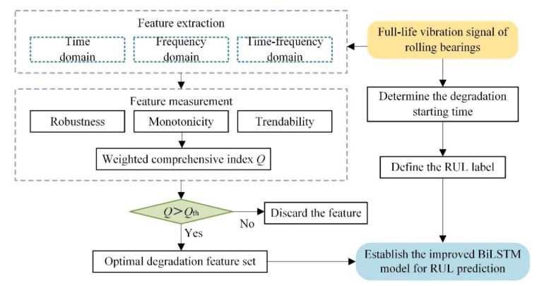
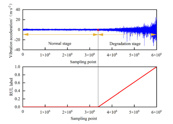
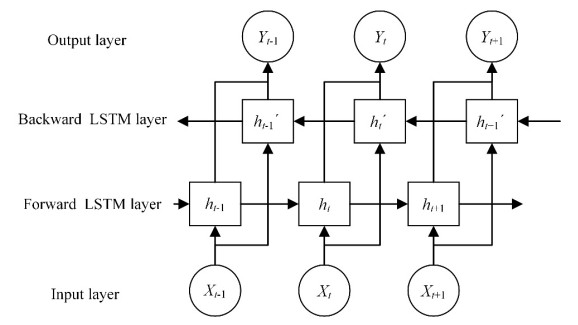
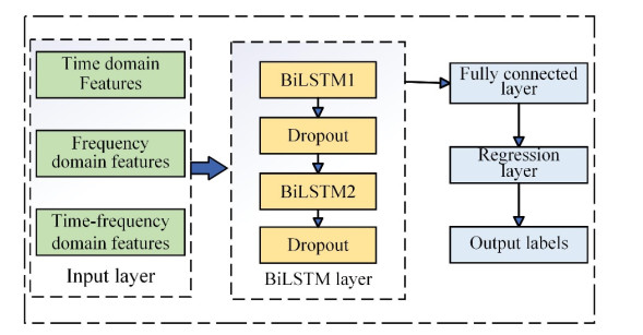
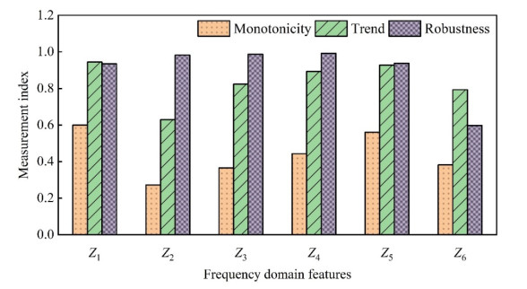
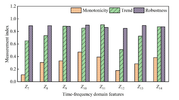
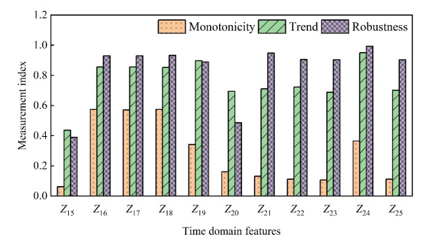
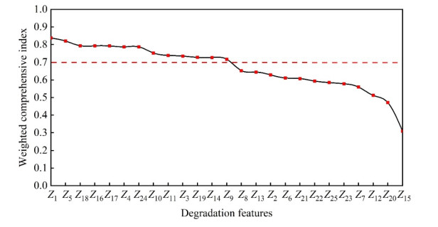
In order to grasp the degradation of rolling bearings and prevent the failure of mechanical equipment, a remaining useful life (RUL) prediction method of rolling bearings based on degradation detection and deep bidirectional long short-term memory networks (BiLSTM) was proposed, considering the incomplete degradation feature extraction and low prediction accuracy of existing methods. By extracting the characteristics of time domain, frequency domain, and time-frequency domain of the full-life bearing vibration signal, the monotonicity, trend, and robustness measurement indexes of each feature were calculated. The best feature set that can fully reflect the degradation information was constructed by ranking the weighted comprehensive indexes of the features. A degradation detection strategy was used to determine the degradation starting time for setting piecewise linear network label. The RUL prediction model based on deep BiLSTM was established and optimized through Dropout technology and piecewise learning rate. The model was verified by the full-life data set of rolling bearings. The results showed that compared with the support vector machine (SVM), the traditional recurrent neural network (RNN), the single-layer BiLSTM, and long short-term memory networks (LSTM) model without Dropout, the proposed method fitted the degradation trend best, and the root mean square error (RMSE) was the smallest and only 0.0281, which improved the accuracy of RUL prediction of rolling bearings, helped prevent bearing failure, and ensured the safe and reliable operation of rotating machinery.
Citation: Shuang Cai, Jiwang Zhang, Cong Li, Zequn He, Zhimin Wang. A RUL prediction method of rolling bearings based on degradation detection and deep BiLSTM[J]. Electronic Research Archive, 2024, 32(5): 3145-3161. doi: 10.3934/era.2024144
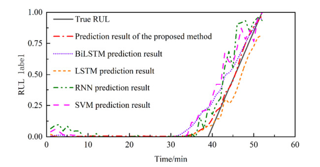
In order to grasp the degradation of rolling bearings and prevent the failure of mechanical equipment, a remaining useful life (RUL) prediction method of rolling bearings based on degradation detection and deep bidirectional long short-term memory networks (BiLSTM) was proposed, considering the incomplete degradation feature extraction and low prediction accuracy of existing methods. By extracting the characteristics of time domain, frequency domain, and time-frequency domain of the full-life bearing vibration signal, the monotonicity, trend, and robustness measurement indexes of each feature were calculated. The best feature set that can fully reflect the degradation information was constructed by ranking the weighted comprehensive indexes of the features. A degradation detection strategy was used to determine the degradation starting time for setting piecewise linear network label. The RUL prediction model based on deep BiLSTM was established and optimized through Dropout technology and piecewise learning rate. The model was verified by the full-life data set of rolling bearings. The results showed that compared with the support vector machine (SVM), the traditional recurrent neural network (RNN), the single-layer BiLSTM, and long short-term memory networks (LSTM) model without Dropout, the proposed method fitted the degradation trend best, and the root mean square error (RMSE) was the smallest and only 0.0281, which improved the accuracy of RUL prediction of rolling bearings, helped prevent bearing failure, and ensured the safe and reliable operation of rotating machinery.

| [1] |
Z. Y. Fan, W. R. Li, K. C. Chang, A bidirectional long short-term memory autoencoder transformer for remaining useful life estimation, Mathematics, 11 (2023), 4972. https://doi.org/10.3390/math11244972 doi: 10.3390/math11244972

|
| [2] |
Y. G. Lei, N. P. Li, L. Guo, N. B. Li, T. Yan, J. Lin, Machinery health prognostics: A systematic review from data acquisition to RUL prediction, Mech. Syst. Signal Process., 104 (2018), 799–834. https://doi.org/10.1016/j.ymssp.2017.11.01 doi: 10.1016/j.ymssp.2017.11.01
|
| [3] |
F. Q. Zhao, Z. G. Tian, Y. Zeng, Uncertainty quantification in gear remaining useful life prediction through an integrated prognostics method, IEEE Trans. Reliab., 62 (2013), 146–159. https://doi.org/10.1109/TR.2013.2241216 doi: 10.1109/TR.2013.2241216
|
| [4] | S. C. Deng, Z. Q. Chen, Z. Chen, Auxiliary particle filter-based remaining useful life prediction of rolling bearing, in 2017 International Conference on Sensing, Diagnostics, Prognostics, and Control (SDPC), (2017), 15–19. |
| [5] |
Y. X. Li, X. Z. Huang, T. H. Gao, C. Y. Zhao, S. J. Li, A wiener-based remaining useful life prediction method with multiple degradation patterns, Adv. Eng. Inf., 57 (2023), 102066. https://doi.org/10.1016/j.aei.2023.102066 doi: 10.1016/j.aei.2023.102066
|
| [6] |
N. P. Li, Y. G. Lei, J. Lin, S. X. Ding, An improved exponential model for predicting remaining useful life of rolling element bearings, IEEE Trans. Ind. Electron., 62 (2015), 7762–7773. https://doi.org/10.1109/TIE.2015.2455055 doi: 10.1109/TIE.2015.2455055
|
| [7] |
A. Rai, S. H. Upadhyay, The use of MD-CUMSUM and NARX neural network for anticipating the remaining useful life of bearings, Measurement, 111 (2017), 397–410. https://doi.org/10.1016/j.measurement.2017.07.030 doi: 10.1016/j.measurement.2017.07.030
|
| [8] |
Z. Liu, M. J. Zuo, Y. Qin, Remaining useful life prediction of rolling element bearings based on health state assessment, Proc. Inst. Mech. Eng., Part C: J. Mech., 230 (2016), 314–330. https://doi.org/10.1177/0954406215590167 doi: 10.1177/0954406215590167
|
| [9] |
F. Deng, Y. Bi, Y. Liu, S. Yang, Deep-learning-based remaining useful life prediction based on a multi-scale dilated convolution network, Mathematics, 9 (2021), 3035. https://doi.org/10.3390/math9233035 doi: 10.3390/math9233035
|
| [10] |
B. Rezaeianjouybari, Y. Shang, Deep learning for prognostics and health management: State of the art, challenges, and opportunities, Measurement, 163 (2020), 107929. https://doi.org/10.1016/j.measurement.2020.107929 doi: 10.1016/j.measurement.2020.107929
|
| [11] |
B. Zhang, S. H. Zhang, W. H. Li, Bearing performance degradation assessment using long short-term memory recurrent network, Comput. Ind., 106 (2019), 14–29. https://doi.org/10.1016/j.compind.2018.12.016 doi: 10.1016/j.compind.2018.12.016
|
| [12] |
Z. H. Chang, W. Yuan, K. Huang, Remaining useful life prediction for rolling bearings using multi-layer grid search and LSTM, Comput. Electr. Eng., 101 (2022), 108083. https://doi.org/10.1016/j.compeleceng.2022.108083 doi: 10.1016/j.compeleceng.2022.108083
|
| [13] |
J. Y. Guo, J. Wang, Z. Y. Wang, Y. Gong, J. L. Qi, G. Y. Wang, et al., A CNN‐BiLSTM‐Bootstrap integrated method for remaining useful life prediction of rolling bearings, Qual. Reliab. Eng. Int., 39 (2023), 1796–1813. https://doi.org/10.1002/qre.3314 doi: 10.1002/qre.3314
|
| [14] |
B. Zhang, L. J. Zhang, J. W. Xu, Degradation feature selection for remaining useful life prediction of rolling element bearings, Qual. Reliab. Eng. Int., 32 (2016), 547–554. https://doi.org/10.1002/qre.1771 doi: 10.1002/qre.1771
|
| [15] |
Y. G. Lei, N. P. Li, S. Gontarz, J. Lin, S. Radkowski, J. Dybala, A model-based method for remaining useful life prediction of machinery, IEEE Trans. Reliab., 65 (2016), 1314–1326. https://doi.org/10.1109/TR.2016.2570568 doi: 10.1109/TR.2016.2570568
|
| [16] |
B. Wang, Y. G. Lei, N. P. Li, N. B. Li, A hybrid prognostics approach for estimating remaining useful life of rolling element bearings, IEEE Trans. Reliab., 69 (2020), 401–412. https://doi.org/10.1109/TR.2018.2882682 doi: 10.1109/TR.2018.2882682
|
Figures(9) / Tables(5)
Shuang Cai, Jiwang Zhang, Cong Li, Zequn He, Zhimin Wang. A RUL prediction method of rolling bearings based on degradation detection and deep BiLSTM[J]. Electronic Research Archive, 2024, 32(5): 3145-3161. doi: 10.3934/era.2024144


 DownLoad: