The effect of innovation performance on the adoption of human resources analytics in business organizations

Eithel F. Bonilla-Chaves; Pedro R. Palos-Sánchez; José A. Folgado-Fernández; Jorge A. Marino-Romero; Eithel F. Bonilla-Chaves; Pedro R. Palos-Sánchez; José A. Folgado-Fernández; Jorge A. Marino-Romero

doi:10.3934/era.2024054

Electronic Research Archive

2024, Volume 32, Issue 2: 1126-1144. doi: 10.3934/era.2024054

Previous Article Next Article

Research article Special Issues

The effect of innovation performance on the adoption of human resources analytics in business organizations

1.
School of Business Administration, Technological Institute of Costa Rica, Cartago 30109, Costa Rica
2.
Department of Financial Economy and Operation Management, University of Sevilla, Sevilla 41018, Spain
3.
Department of Financial Economy and Accounting, Universidad de Extremadura, Cáceres 10071, Spain

Received: 02 October 2023 Revised: 15 December 2023 Accepted: 08 January 2024 Published: 25 January 2024

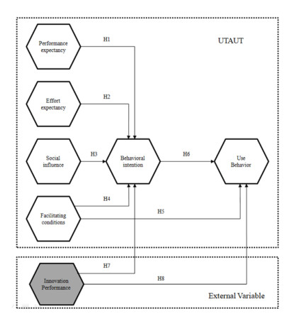
Our study objective is to examine the determinants that influence the adoption of human resource (HR) analytics, along with the influence of the external variable called Innovation Performance. The research model was developed by adapting the theoretical model of the unified theory of the acceptance and use of technology (UTAUT) by adding the external variable, Innovation Performance. The data was collected using a survey at Amazon Mechanical Turk (MTurk) in the USA. Initially, a total of 602 responses were obtained. Finally, a total of 554 questionnaires were obtained after using information quality filters for debugging. This study reveals that the main influence on the adoption of HR analytics is exerted by performance expectancy, social influence, facilitating conditions, and innovation performance on behavioral intention. Likewise, facilitating conditions, innovative performance, and behavior intention are the major influences for Use Behavior. This was found from an empirical analysis using the generalized structured component analysis (GSCA) software package that shows, with tabled data, the major relationships of the research model. This research into the use of HR Analytics investigated the standard determinants of UTAUT and the Innovation Performance external variable, that influence the adoption of HR analytics in business organization.

Keywords:

Citation: Eithel F. Bonilla-Chaves, Pedro R. Palos-Sánchez, José A. Folgado-Fernández, Jorge A. Marino-Romero. The effect of innovation performance on the adoption of human resources analytics in business organizations[J]. Electronic Research Archive, 2024, 32(2): 1126-1144. doi: 10.3934/era.2024054

Related Papers:

[1]	Hatim Solayman Migdadi, Nesreen M. Al-Olaimat, Maryam Mohiuddin, Omar Meqdadi . Statistical inference for the Power Rayleigh distribution based on adaptive progressive Type-II censored data. AIMS Mathematics, 2023, 8(10): 22553-22576. doi: 10.3934/math.20231149
[2]	M. G. M. Ghazal . Modified Chen distribution: Properties, estimation, and applications in reliability analysis. AIMS Mathematics, 2024, 9(12): 34906-34946. doi: 10.3934/math.20241662
[3]	Azam Zaka, Ahmad Saeed Akhter, Riffat Jabeen . The new reflected power function distribution: Theory, simulation & application. AIMS Mathematics, 2020, 5(5): 5031-5054. doi: 10.3934/math.2020323
[4]	H. M. Barakat, M. A. Alawady, I. A. Husseiny, M. Nagy, A. H. Mansi, M. O. Mohamed . Bivariate Epanechnikov-exponential distribution: statistical properties, reliability measures, and applications to computer science data. AIMS Mathematics, 2024, 9(11): 32299-32327. doi: 10.3934/math.20241550
[5]	Fiaz Ahmad Bhatti, G. G. Hamedani, Mashail M. Al Sobhi, Mustafa Ç. Korkmaz . On the Burr XII-Power Cauchy distribution: Properties and applications. AIMS Mathematics, 2021, 6(7): 7070-7092. doi: 10.3934/math.2021415
[6]	Ekramy A. Hussein, Hassan M. Aljohani, Ahmed Z. Afify . The extended Weibull–Fréchet distribution: properties, inference, and applications in medicine and engineering. AIMS Mathematics, 2022, 7(1): 225-246. doi: 10.3934/math.2022014
[7]	Hisham Mahran, Mahmoud M. Mansour, Enayat M. Abd Elrazik, Ahmed Z. Afify . A new one-parameter flexible family with variable failure rate shapes: Properties, inference, and real-life applications. AIMS Mathematics, 2024, 9(5): 11910-11940. doi: 10.3934/math.2024582
[8]	M. G. M. Ghazal, Yusra A. Tashkandy, Oluwafemi Samson Balogun, M. E. Bakr . Exponentiated extended extreme value distribution: Properties, estimation, and applications in applied fields. AIMS Mathematics, 2024, 9(7): 17634-17656. doi: 10.3934/math.2024857
[9]	Haidy A. Newer, Mostafa M. Mohie El-Din, Hend S. Ali, Isra Al-Shbeil, Walid Emam . Statistical inference for the Nadarajah-Haghighi distribution based on ranked set sampling with applications. AIMS Mathematics, 2023, 8(9): 21572-21590. doi: 10.3934/math.20231099
[10]	Alaa M. Abd El-Latif, Hanan H. Sakr, Mohamed Said Mohamed . Fractional generalized cumulative residual entropy: properties, testing uniformity, and applications to Euro Area daily smoker data. AIMS Mathematics, 2024, 9(7): 18064-18082. doi: 10.3934/math.2024881

Abstract

1. Introduction

In numerous practical situations, the datasets are measured in the number of cycles, runs, and/or shocks the device sustains before its failure. For example, the number of voltage fluctuations, the lifetime of a discrete random variable (rv), and frequency of a device switched on/off, the life of a weapon is measured by the number of rounds fired before failure, and the number of completed cycles measures the life of the equipment. Further, the number of patients, number of deaths due to a disease/virus, and number of days a patient stays in a hospital ward. Various discrete probability models can be adopted to analyze such types of datasets.

The well-known traditional discrete probability models, including the negative binomial, geometric, and Poisson distributions have limitations to use due to their specific behavior such as the Poisson distribution that performs better with datasets having dispersion equal to average; the NB distribution is applicable for over-dispersed datasets. The real-life datasets may be over-dispersed or under-dispersed, so there is always a clear need for flexible discrete distributions to have a good resolution.

Several discretized forms of continuous distributions have been derived to model different count datasets in the last few decades. The most notable discretization approach in the literature is the survival discretizing approach which has gained much attention.

Let rv $X$ follows a continuous distribution with survival function (sf) $S\left(x\right)$ . Using the survival discretization approach introduced by Kemp (2004), the probability mass function (pmf) of a discrete rv follows as

$p\left(x\right) = P\left(X = x\right) = S\left(x\right)-S\left(x+1\right), \;\;\;\;x = \mathrm{0, 1}, \mathrm{2, 3}, \dots$

(1)

The survival discretization approach has been adopted to develop many discrete models. For example, the discrete normal ^[1], discrete Rayleigh ^[2], discrete half-normal ^[3], discrete Burr and discrete Pareto ^[4], discrete inverse-Weibull ^[5], new generalization of the geometric ^[6], discrete Lindley ^[7], generalized exponential type Ⅱ ^[8], discrete inverse-Rayleigh ^[9], two-parameter discrete Lindley ^[10], discrete log-logistic ^[11], discrete extended Weibull ^[12], exponentiated discrete-Lindley ^[13], discrete Burr-Hutke ^[14], discrete Marshall-Olkin Weibull ^[15], natural discrete-Lindley ^[16], discrete Bilal ^[17], discrete inverted Topp-Leone ^[18], uniform Poisson–Ailamujia ^[19], exponentiated discrete Lindley ^[20], discrete exponentiated Burr–Hatke ^[21], discrete Ramos-Louzada ^[22] and ^[23], and discrete type-Ⅱ half-logistic exponential ^[24].

The main goal of the present study is to introduce a new discrete distribution to model over-dispersed as well as under-dispersed datasets. The proposed distribution is called the discrete power-Ailamujia (DsPA) distribution. The mathematical properties of the DsPA distribution are derived and its parameters are estimated using the maximum likelihood method. Three real count datasets are fitted using the DsPA model and other competing discrete distributions. The DsPA distribution provides a better fit to the three datasets than some well-known discrete models according to the results of the simulation.

The paper is organized in the following sections. Section 2 is devoted to the derivation of the new DsPA distribution. Its mathematical properties are explored in Section 3. Section 4 is devoted to estimating the DsPA parameters and providing a comprehensive simulation study. The usefulness of the DsPA distribution is addressed in Section 5. Finally, we conclude the study in Section 6.

2. The DsPA distribution

Jamal et al. ^[25] proposed a new continuous lifetime distribution called the power-Ailamujia distribution. Its probability density function and sf can be expressed as

$f\left(x\right) = {\theta }^{2}{\beta x}^{2\beta -1}{e}^{-\theta {x}^{\beta }}, \;\;\;\;x\ge 0, \theta , \beta > 0$

(2)

and

$S\left(x\right) = \left(1+\theta {x}^{\beta }\right){e}^{-\theta {x}^{\beta }}, \;\;\;\;x\ge 0, \theta , \beta > 0,$

(3)

respectively.

Applying the survival discretization approach in (1), the rv $X$ is said to have the DsPA distribution with parameters $0 < \lambda < 1$ and $\beta > 0,$ if its sf takes the form

$S\left(x;\lambda , \beta \right) = {\lambda }^{{\left(x+1\right)}^{\beta }}\left[1-{\left(x+1\right)}^{\beta }\mathrm{ln}\lambda \right], \;\;\;\;x\in {\mathbb{N}}_{0},$

(4)

where $\lambda = {e}^{-\theta }$ and ${\mathbb{N}}_{0} = \left\{0, 1, 2, \dots , w\right\}$ for $0 < w < \infty$ .

The corresponding cumulative distribution function (cdf) and pmf can be expressed as

$F\left(x;\lambda , \beta \right) = 1-{\lambda }^{{\left(x+1\right)}^{\beta }}\left[1-{\left(x+1\right)}^{\beta }\mathrm{ln}\lambda \right], \;\;\;\;x\in {\mathbb{N}}_{0}$

(5)

and

${P}_{x}\left(x;\lambda \right) = {\lambda }^{{x}^{\beta }}\left[1-{x}^{\beta }ln\lambda \right]-{\lambda }^{{\left(x+1\right)}^{\beta }}\left[1-{\left(x+1\right)}^{\beta }\mathrm{ln}\lambda \right], \;\;\;\;x\in {\mathbb{N}}_{0}.$

(6)

Plots of the DsPA pmf, for various values of the parameters $\lambda$ and $\beta$ , are presented in Figure 1.

Figure 1. Shapes of the DsPA pmf for some values of

$\lambda$ and

$\beta$ .

DownLoad: Full-Size Img PowerPoint

The hazard rate function (hrf) of the DsPA distribution can be expressed as

$h\left(x;\lambda \right) = \frac{p\left(x\right)}{S\left(x\right)} = \frac{{\lambda }^{{x}^{\beta }}\left[1-{x}^{\beta }ln\lambda \right]}{{\lambda }^{{\left(x+1\right)}^{\beta }}\left[1-{\left(x+1\right)}^{\beta }\mathrm{ln}\lambda \right]}-1, \;\;\;\;x\in {\mathbb{N}}_{0}$

(7)

where $h\left(x;\lambda \right) = \frac{P\left(x\right)}{S\left(x\right)}.$ shows the DsPA hrf plots for different values of $\lambda$ and $\beta$ .

Figure 2. Shapes of the DsPA hrf for some values of

$\lambda$ and

$\beta$ .

DownLoad: Full-Size Img PowerPoint

The quantile function of the DsPA distribution reduces to

$Q\left( u \right) = \left\lfloor {1 - \left[ {1 - {{\left( {x + 1} \right)}^\beta }{\rm{ln}}\lambda } \right]{\lambda ^{{{\left( {x + 1} \right)}^\beta }}}} \right\rfloor , 0 < u < 1,$

where $\left\lfloor x \right\rfloor$ denotes the integer part of $x$ .

The reverse hrf (rhrf) of the DsPA distribution is defined as

${r}^{*}\left(x\right) = \frac{p\left(x\right)}{F\left(x\right)} = \frac{{\lambda }^{{x}^{\beta }}\left[1-{x}^{\beta }ln\lambda \right]-{\lambda }^{{\left(x+1\right)}^{\beta }}\left[1-{\left(x+1\right)}^{\beta }\mathrm{ln}\lambda \right]}{1-{\lambda }^{{\left(x+1\right)}^{\beta }}\left[1-{\left(x+1\right)}^{\beta }\mathrm{ln}\lambda \right]}, \;\;\;\;\; x\in {\mathbb{N}}_{0},$

(8)

where ${r}^{*}\left(x\right) = \frac{P\left(x\right)}{F\left(x\right)}.$ shows the DsPA rhrf plots for several values of $\lambda$ and $\beta$ .

Figure 3. Possible shapes of the DsPA rhrf for several values of

$\lambda$ and

$\beta$ .

DownLoad: Full-Size Img PowerPoint

The second failure rate of the DsPA distribution is expressed by

${r}^{**}\left(x\right) = \mathrm{log}\left\{\frac{S\left(x\right)}{S\left(x+1\right)}\right\} = \mathrm{log}\left\{\frac{{\lambda }^{{\left(x+1\right)}^{\beta }}\left[1-{\left(x+1\right)}^{\beta }\mathrm{ln}\lambda \right]}{{\lambda }^{{\left(x+2\right)}^{\beta }}\left[1-{\left(x+2\right)}^{\beta }\mathrm{ln}\lambda \right]}\right\}, \;\;\;\;\;x\in {\mathbb{N}}_{0}.$

(9)

The recurrence relation of probabilities from the DsPA distribution has the form

$\frac{P\left(x+1\right)}{P\left(x\right)} = \frac{{\lambda }^{{\left(x+1\right)}^{\beta }}\left[1-{\left(x+1\right)}^{\beta }ln\lambda \right]-{\lambda }^{{\left(x+2\right)}^{\beta }}\left[1-{\left(x+2\right)}^{\beta }\mathrm{ln}\lambda \right]}{{\lambda }^{{x}^{\beta }}\left[1-{x}^{\beta }ln\lambda \right]-{\lambda }^{{\left(x+1\right)}^{\beta }}\left[1-{\left(x+1\right)}^{\beta }\mathrm{ln}\lambda \right]}.$

(10)

Hence,

$P\left(x+1\right) = \frac{{\lambda }^{{\left(x+1\right)}^{\beta }}\left[1-{\left(x+1\right)}^{\beta }ln\lambda \right]-{\lambda }^{{\left(x+2\right)}^{\beta }}\left[1-{\left(x+2\right)}^{\beta }\mathrm{ln}\lambda \right]}{{\lambda }^{{x}^{\beta }}\left[1-{x}^{\beta }ln\lambda \right]-{\lambda }^{{\left(x+1\right)}^{\beta }}\left[1-{\left(x+1\right)}^{\beta }\mathrm{ln}\lambda \right]}P\left(x\right).$

3. Some properties of the DsPA distribution

In this section, we studied some mathematical properties of the DsPA distribution. In this section, we studied some mathematical properties of the DsPA distribution.

3.1. Moments and generating functions

The probability generating function (pgf) of the DsPA distribution is given as follows

${G}_{x}\left(z\right) = 1\mathrm{ }+\mathrm{ }(z-1)\sum \limits_{x = 1}^{\infty }{z}^{x-1}\left(1-{x}^{\beta }\mathrm{l}\mathrm{n}\lambda \right){\lambda }^{{x}^{\beta }},$

(11)

where ${G}_{x}\left(z\right) = \sum _{x = 0}^{\infty }{z}^{x}P\left(x\right)$ . The moment generating function (mgf) can be obtained by replacing z with ${e}^{z}$ in Eq (11). Thus, the mgf of the DsPA distribution can be expressed as

${M}_{x}\left(z\right) = 1\mathrm{ }+\mathrm{ }({e}^{z}-1)\sum \limits_{x = 1}^{\infty }{\left({e}^{z}\right)}^{x-1}\left(1-{x}^{\beta }\mathrm{l}\mathrm{n}\lambda \right){\lambda }^{{x}^{\beta }}.$

(12)

Thus, the first four moments of the DsPA distribution are

$E\left(X\right) = \sum \limits_{x = 1}^{\infty }\left(1-{x}^{\beta }\mathrm{l}\mathrm{n}\lambda \right){\lambda }^{{x}^{\beta }},$

(13)

$E\left({X}^{2}\right) = \sum \limits_{x = 1}^{\infty }(2x-1)\left(1-{x}^{\beta }\mathrm{l}\mathrm{n}\lambda \right){\lambda }^{{x}^{\beta }},$

$E\left({X}^{3}\right) = \sum \limits_{x = 1}^{\infty }\left(3{x}^{2}-3x+1\right)\left(1-{x}^{\beta }\mathrm{l}\mathrm{n}\lambda \right){\lambda }^{{x}^{\beta }}$

and

$E\left({X}^{4}\right) = \sum \limits_{x = 1}^{\infty }\left(4{x}^{3}-6{x}^{2}+4x-1\right)\left(1-{x}^{\beta }\mathrm{l}\mathrm{n}\lambda \right){\lambda }^{{x}^{\beta }}.$

Using the above moments, the variance ( ${\sigma }^{2}$ ), coefficient of skewness (CS), and coefficient of kurtosis (CK) can be presented in closed-form expressions. Further, another classical concept, called dispersion index (DI). The DI is defined as a variance to mean ratio. If the DI value is less than 1, then the model is suitable for under-dispersed datasets. Conversely, if the DI is greater than 1, then it is suitable for over-dispersed datasets. Numerical values of the mean, $E\left(X\right),$ ${\sigma }^{2},$ CS, CK and DI are reported in Tables 1‒5.

Table 1. Numerical values for the mean of the DsPA model.

$\mathit{\boldsymbol{\beta }}$	$\mathit{\boldsymbol{\lambda }}$
$\mathit{\boldsymbol{\beta }}$	0.1	0.2	0.3	0.4	0.5	0.6	0.7	0.8	0.9
0.5	0.7603	1.8909	3.6766	6.5446	10.966	16.848	22.277	22.458	12.187
1.0	0.3954	0.7529	1.1657	1.6848	2.3863	3.4156	5.1075	8.4629	18.452
1.5	0.3415	0.5827	0.8221	1.0907	1.4187	1.8533	2.4910	3.5895	6.2446
2.0	0.3313	0.5338	0.7085	0.8884	1.0967	1.3599	1.7259	2.3141	3.5954
2.5	0.3303	0.5230	0.6698	0.8012	0.9444	1.1259	1.3763	1.7634	2.5557
3.0	0.3303	0.5219	0.6619	0.7720	0.8721	0.9919	1.1725	1.4628	2.0209

| Show Table

DownLoad: CSV

Table 2. Numerical values for the variance of the DsPA model.

$\mathit{\boldsymbol{\beta }}$	$\mathit{\boldsymbol{\lambda }}$
$\mathit{\boldsymbol{\beta }}$	0.1	0.2	0.3	0.4	0.5	0.6	0.7	0.8	0.9
0.5	2.7920	12.243	38.665	103.06	229.88	417.28	621.34	779.36	615.37
1.0	0.3901	0.8140	1.4378	2.4502	4.2371	7.7429	15.802	40.249	177.94
1.5	0.2475	0.3692	0.4988	0.6724	0.9299	1.3485	2.1203	3.8858	10.421
2.0	0.2236	0.2727	0.3017	0.3478	0.4232	0.5408	0.7369	1.1271	2.2935
2.5	0.2213	0.2517	0.2384	0.2287	0.2486	0.3033	0.3864	0.5260	0.8911
3.0	0.2212	0.2496	0.2252	0.1869	0.1626	0.1789	0.2448	0.3256	0.4729

| Show Table

DownLoad: CSV

Table 3. Numerical values for the skewness of the DsPA model.

$\mathit{\boldsymbol{\beta }}$	$\mathit{\boldsymbol{\lambda }}$
$\mathit{\boldsymbol{\beta }}$	0.1	0.2	0.3	0.4	0.5	0.6	0.7	0.8	0.9
0.5	4.6187	4.3533	3.9822	3.2831	2.4657	1.7555	1.2590	1.1461	2.0439
1.0	1.6228	1.4038	1.3664	1.3697	1.3821	1.3943	1.4037	1.4099	1.3511
1.5	0.9461	0.5856	0.5417	0.5744	0.6191	0.6586	0.6895	0.7124	0.7285
2.0	0.7459	0.1163	-0.0092	0.1018	0.2223	0.2912	0.3312	0.3598	0.3836
2.5	0.7226	-0.0655	-0.4988	-0.4984	-0.1012	0.1683	0.1697	0.1591	0.1742
3.0	0.7218	-0.0869	-0.6648	-1.0922	-0.9663	-0.0481	0.3705	0.0738	0.0476

| Show Table

DownLoad: CSV

Table 4. Numerical values for the kurtosis of the DsPA model.

$\mathit{\boldsymbol{\beta }}$	$\mathit{\boldsymbol{\lambda }}$
$\mathit{\boldsymbol{\beta }}$	0.1	0.2	0.3	0.4	0.5	0.6	0.7	0.8	0.9
0.5	41.471	36.784	28.534	18.030	10.188	5.7950	3.7130	3.1485	5.9942
1.0	5.9572	5.6739	5.7391	5.8240	5.8909	5.9380	5.9690	5.9875	5.4737
1.5	2.5630	2.7503	3.1474	3.3764	3.4912	3.5508	3.5857	3.6093	3.6262
2.0	1.6369	1.5891	2.4907	3.0833	3.1595	3.0954	3.0599	3.0514	3.0542
2.5	1.5246	1.0744	1.8108	3.2354	3.9993	3.4076	2.8767	2.8838	2.8977
3.0	1.5211	1.0098	1.4967	2.7867	4.9278	5.5909	3.4605	2.4008	2.8802

| Show Table

DownLoad: CSV

Table 5. Numerical values for the DI of the DsPA model.

$\mathit{\boldsymbol{\beta }}$	$\mathit{\boldsymbol{\lambda }}$
$\mathit{\boldsymbol{\beta }}$	0.1	0.2	0.3	0.4	0.5	0.6	0.7	0.8	0.9
0.5	3.6720	6.4746	10.516	15.747	20.964	24.768	27.891	34.703	50.494
1.0	0.9866	1.0810	1.2335	1.4543	1.7756	2.2669	3.0939	4.7559	9.6437
1.5	0.7248	0.6337	0.6068	0.6165	0.6555	0.7276	0.8512	1.0826	1.6688
2.0	0.6749	0.5109	0.4258	0.3915	0.3859	0.3977	0.4269	0.4870	0.6379
2.5	0.6699	0.4813	0.3559	0.2854	0.2632	0.2694	0.2808	0.2983	0.3487
3.0	0.6697	0.4782	0.3402	0.2422	0.1865	0.1804	0.2088	0.2226	0.2340

| Show Table

DownLoad: CSV

From ‒, we can conclude that the mean is an increasing function of $\lambda$ and a decreasing function of $\beta$ . It is clear that the skewness of the DsPA distribution can be positive or negative. The DI showing increasing behavior for larger values of the parameter $\lambda$ and small values of $\beta$ . Further, the DsPA distribution is suitable for over-dispersed and under-dispersed data sets.

3.2. Mean Residual Life (MRL)

The MRL function is a helpful reliability characteristic to model and analyze the burn-in and maintenance policies. Consider the rv $X$ that has the cdf $F\left(.\right)$ . For a discrete rv, the MRL function is defined by

$MRL = \varepsilon \left(i\right) = E\left(X-i|X\ge i\right) = \frac{1}{1-F\left(i-1, \lambda \right)}\sum \limits_{j = i+1}^{w}\left[1-F\left(j-1, \lambda \right)\right], \;\;\;\;i\in {\mathbb{N}}_{0},$

where ${\mathbb{N}}_{0} = \left\{0, 1, 2, \dots , w\right\}$ and $0 < w < \infty$ .

Then, the MRL of the DsPA model reduces to

$MRL = \frac{1}{1-F\left(i-1, \lambda , \beta \right)}\sum \limits_{j = i+1}^{w}\left[1-F\left(j-1, \lambda , \beta \right)\right]$

$= \frac{1}{\left[1-{\left(i\right)}^{\beta }\mathrm{ln}\lambda \right]{\lambda }^{{\left(i\right)}^{\beta }}}\sum \limits_{j = i+1}^{w}\left[1-{\left(j\right)}^{\beta }\mathrm{ln}\lambda \right]{\lambda }^{{\left(j\right)}^{\beta }}$

$= \frac{1}{\left[1-{\left(i\right)}^{\beta }\mathrm{ln}\lambda \right]{\lambda }^{{\left(i\right)}^{\beta }}}\left[\sum \limits_{j = i+1}^{w}{\lambda }^{{\left(j\right)}^{\beta }}-\mathrm{ln}\lambda \sum \limits_{j = i+1}^{w}{\left(j\right)}^{\beta }{\lambda }^{{\left(j\right)}^{\beta }}\right].$

4. Parameter estimation

In this section, the parameters λ and β are estimated using the maximum likelihood (ML) method.

4.1. Maximum likelihood estimation

Suppose ${x}_{1}, \dots , {x}_{n}$ be a random sample from the DsPA distribution with pmf (6). Then the log-likelihood function takes the form

$L = \frac{1}{\left[1-{\left(i\right)}^{\beta }\mathrm{ln}\lambda \right]{\lambda }^{{\left(i\right)}^{\beta }}}\sum \limits_{j = i+1}^{w}\left[1-{\left(j\right)}^{\beta }\mathrm{ln}\lambda \right]{\lambda }^{{\left(j\right)}^{\beta }}.$

(14)

Now, by differentiating (14) w.r.t $\lambda$ and $\beta$ , we can write

$\frac{\partial L}{\partial \lambda } = \sum \limits_{i = 1}^{n}\frac{\mathrm{ln}\lambda \left[{\left({x}_{i}+1\right)}^{2\beta }{\lambda }^{{\left({x}_{i}+1\right)}^{\beta }}-{{x}_{i}}^{2\beta }{\lambda }^{{{x}_{i}}^{\beta }}\right]}{\lambda \left\{\left[1-{{x}_{i}}^{\beta }\mathrm{l}\mathrm{n}\lambda \right]{\lambda }^{{{x}_{i}}^{\beta }}-\left[1-{\left({x}_{i}+1\right)}^{\beta }\mathrm{ln}\lambda \right]{\lambda }^{{\left({x}_{i}+1\right)}^{\beta }}\right\}} = 0$

(15)

and

$\frac{\partial L}{\partial \beta } = \sum \limits_{i = 1}^{n}\frac{{\left(\mathrm{ln}\lambda \right)}^{2}\left[{\lambda }^{{\left({x}_{i}+1\right)}^{\beta }}{\left({x}_{i}+1\right)}^{2\beta }\mathrm{ln}({x}_{i}+1)-{\lambda }^{{{x}_{i}}^{\beta }}{{x}_{i}}^{2\beta }\mathrm{ln}{x}_{i}\right]}{\left\{\left[1-{{x}_{i}}^{\beta }\mathrm{l}\mathrm{n}\lambda \right]{\lambda }^{{{x}_{i}}^{\beta }}-\left[1-{\left({x}_{i}+1\right)}^{\beta }\mathrm{ln}\lambda \right]{\lambda }^{{\left({x}_{i}+1\right)}^{\beta }}\right\}} = 0.$

(16)

The ML estimates (MLEs) of $\lambda$ and $\beta$ follow from the above equation. Eqs (15) and (16) can be solved using iterative procedures such as Newton-Raphson. For this purpose, we use the maxLik function of R software ^[26].

4.2. Simulation study

In this section, we carried out a numerical simulation to access the performance of the ML estimation method. This assessment is done by generating $N = \mathrm{10,000}$ samples using the qf of the DsPA model for different sample sizes $n = 10, 20, 50,$ and $100$ and for several values of the parameters $\lambda$ and $\beta$ , where $\left(\lambda , \beta \right) = \left(0.50, 0.50\right), \left(0.50, 2.0\right), \left(0.90, 1.20\right), (0.90, 2.0).$ The assessment is completed using absolute bias, mean relative errors (MREs), and mean square errors (MSEs) which are defined by

$Bias\left(\mathit{\boldsymbol{\delta }}\right) = \frac{1}{N}\sum \limits_{i = 1}^{N}\left|{\widehat{\mathit{\boldsymbol{\delta }}}}_{i}-\mathit{\boldsymbol{\delta }}\right|, MSE\left(\mathit{\boldsymbol{\delta }}\right) = \frac{1}{N}\sum \limits_{i = 1}^{N}{\left({\widehat{\mathit{\boldsymbol{\delta }}}}_{i}-\mathit{\boldsymbol{\delta }}\right)}^{2}\;\mathrm{a}\mathrm{n}\mathrm{d}\;MRE\left(\mathit{\boldsymbol{\delta }}\right) = \frac{1}{N}\sum \limits_{i = 1}^{N}\frac{{\widehat{\mathit{\boldsymbol{\delta }}}}_{i}}{{\mathit{\boldsymbol{\delta }}}_{i}},$

where $\mathit{\boldsymbol{\delta }} = (\lambda$ , $\beta ).$

The simulation results for $\lambda$ and $\beta$ are reported in ‒. The bias, MSE and MRE of the parameters $\lambda$ and $\beta$ are computed using the R program using the ML method. For all values of $\lambda$ and $\beta$ , the ML estimation approach illustrates the consistency property, that is, the MSEs and MREs decrease as $n$ increases.

Table 6. Simulation results of the DsPA distribution for

$\lambda = 0.5$ and

$\beta = 0.5$ .

$n$	$E\left(\lambda \right)$	$E\left(\beta \right)$	$\mathrm{B}\mathrm{i}\mathrm{a}\mathrm{s}\left(\lambda \right)$	$\mathrm{B}\mathrm{i}\mathrm{a}\mathrm{s}\left(\beta \right)$	$\mathrm{M}\mathrm{S}\mathrm{E}\left(\lambda \right)$	$\mathrm{M}\mathrm{S}\mathrm{E}\left(\beta \right)$	$\mathrm{M}\mathrm{R}\mathrm{E}\left(\lambda \right)$	$\mathrm{M}\mathrm{R}\mathrm{E}\left(\beta \right)$
10	0.4605	0.5804	-0.0395	0.0804	0.0483	0.0333	0.0789	0.1609
20	0.4796	0.5370	-0.0204	0.0370	0.0247	0.0111	0.0409	0.0740
50	0.4910	0.5143	-0.0090	0.0143	0.0098	0.0033	0.0180	0.0286
100	0.4966	0.5065	-0.0034	0.0065	0.0049	0.0015	0.0069	0.0130
200	0.4975	0.5037	-0.0025	0.0037	0.0024	0.0007	0.0050	0.0074

| Show Table

DownLoad: CSV

Table 7. Simulation results of the DsPA distribution for

$\lambda = 0.5$ and

$\beta = 2.0$ .

$n$	$E\left(\lambda \right)$	$E\left(\beta \right)$	$\mathrm{B}\mathrm{i}\mathrm{a}\mathrm{s}\left(\lambda \right)$	$\mathrm{B}\mathrm{i}\mathrm{a}\mathrm{s}\left(\beta \right)$	$\mathrm{M}\mathrm{S}\mathrm{E}\left(\lambda \right)$	$\mathrm{M}\mathrm{S}\mathrm{E}\left(\beta \right)$	$\mathrm{M}\mathrm{R}\mathrm{E}\left(\lambda \right)$	$\mathrm{M}\mathrm{R}\mathrm{E}\left(\beta \right)$
10	0.4654	2.3160	-0.0346	0.3160	0.0490	0.5537	0.0692	0.1580
20	0.4809	2.1419	-0.0191	0.1419	0.0243	0.1730	0.0382	0.0709
50	0.4905	2.0571	-0.0095	0.0571	0.0097	0.0514	0.0191	0.0286
100	0.4970	2.0243	-0.0030	0.0243	0.0050	0.0247	0.0060	0.0122
200	0.4984	2.0125	-0.0016	0.0125	0.0024	0.0115	0.0032	0.0062

| Show Table

DownLoad: CSV

Table 8. Simulation results of the DsPA distribution for

$\lambda = 0.9$ and

$\beta = 1.2$ .

$n$	$E\left(\lambda \right)$	$E\left(\beta \right)$	$\mathrm{B}\mathrm{i}\mathrm{a}\mathrm{s}\left(\lambda \right)$	$\mathrm{B}\mathrm{i}\mathrm{a}\mathrm{s}\left(\beta \right)$	$\mathrm{M}\mathrm{S}\mathrm{E}\left(\lambda \right)$	$\mathrm{M}\mathrm{S}\mathrm{E}\left(\beta \right)$	$\mathrm{M}\mathrm{R}\mathrm{E}\left(\lambda \right)$	$\mathrm{M}\mathrm{R}\mathrm{E}\left(\beta \right)$
10	0.8630	1.3915	-0.0370	0.1915	0.0990	0.1973	0.0411	0.1596
20	0.8843	1.2834	-0.0157	0.0834	0.0473	0.0630	0.0174	0.0695
50	0.8926	1.2310	-0.0074	0.0310	0.0181	0.0190	0.0082	0.0258
100	0.8972	1.2154	-0.0028	0.0154	0.0088	0.0086	0.0031	0.0129
200	0.8980	1.2076	-0.0020	0.0076	0.0045	0.0043	0.0022	0.0063

| Show Table

DownLoad: CSV

From Tables 6‒8, we conclude that:

1. The estimates of $\lambda$ and $\beta$ close to their true values with the increase of $n$ for all studied cases.

2. The MSEs for $\lambda$ and $\beta$ decrease with the increase of $n$ for all studied cases.

3. The MREs for $\lambda$ and $\beta$ decrease with the increase of $n$ for all studied cases.

Table 9. Simulation results of the DsPA distribution for

$\lambda = 0.9$ and

$\beta = 2.0$ .

$n$	$E\left(\lambda \right)$	$E\left(\beta \right)$	$\mathrm{B}\mathrm{i}\mathrm{a}\mathrm{s}\left(\lambda \right)$	$\mathrm{B}\mathrm{i}\mathrm{a}\mathrm{s}\left(\beta \right)$	$\mathrm{M}\mathrm{S}\mathrm{E}\left(\lambda \right)$	$\mathrm{M}\mathrm{S}\mathrm{E}\left(\beta \right)$	$\mathrm{M}\mathrm{R}\mathrm{E}\left(\lambda \right)$	$\mathrm{M}\mathrm{R}\mathrm{E}\left(\beta \right)$
10	0.8690	2.3159	-0.0310	0.3159	0.1005	0.5381	0.0344	0.1580
20	0.8785	2.1443	-0.0215	0.1443	0.0454	0.1699	0.0239	0.0722
50	0.8941	2.0523	-0.0059	0.0523	0.0183	0.0535	0.0065	0.0261
100	0.8957	2.0278	-0.0043	0.0278	0.0089	0.0246	0.0048	0.0139
200	0.8980	2.0139	-0.0020	0.0139	0.0044	0.0117	0.0022	0.0070

| Show Table

DownLoad: CSV

5. Three real-life applications

In this section, we illustrate the importance of the newly DsPA distribution by utilizing three real-life datasets. We shall compare the fits of the DsPA distribution with the following competing discrete distributions which are reported in Table 10.

Table 10. The competing discrete models of the DsPA distribution with their pmfs.

Model	Abbreviation	pmf
Discrete Bur-Ⅻ	DsBⅫ	$P\left(x\right)={\lambda }^{\mathrm{ln}\left(1+{x}^{\alpha }\right)}-{\lambda }^{\mathrm{ln}\left(1+{\left(1+x\right)}^{\alpha }\right)}.$
Uniform Poisson–Ailamujia	UPA	$P\left(x\right)=2\lambda {(1+2\lambda )}^{-x-1}.$
Poisson	Poi	$P\left(x\right)=\frac{{e}^{-\lambda }{\lambda }^{x}}{x!}.$
Discrete-Pareto	DsPr	$P\left(x\right)={e}^{-\lambda \mathrm{ln}\left(1+x\right)}-{e}^{-\lambda \mathrm{ln}\left(2+x\right)}.$
Discrete-Rayleigh	DsR	$P\left(x\right)={e}^{-\frac{{x}^{2}}{2{\lambda }^{2}}}-{e}^{-\frac{{\left(x+1\right)}^{2}}{2{\lambda }^{2}}}.$
Discrete inverse-Rayleigh	DsIR	$P\left(x\right)={e}^{-\frac{\lambda }{{(1+x)}^{2}}}-{e}^{-\frac{\lambda }{{x}^{2}}}.$
Discrete Burr-Hutke	DsBH	$P\left(x\right)=\left(\frac{1}{x+1}-\frac{\lambda }{x+2}\right){\lambda }^{x}.$

| Show Table

DownLoad: CSV

The fitted distributions are compared using the negative maximum log-likelihood (-Loglik.), Akaike information criterion (AIC), Bayesian information criterion (BIC), and the p-value of Kolmogorov–Smirnov test (KS p-value).

Dataset Ⅰ: The first dataset is about the failure times for a sample of 15 electronic components in an acceleration life test ^[27]. The data observations are: 1.0, 5.0, 6.0, 11.0, 12.0, 19.0, 20.0, 22.0, 23.0, 31.0, 37.0, 46.0, 54.0, 60.0 and 66.0.

Dataset Ⅱ: The second dataset is about the number of fires in Greece from July 1, 1998 to August 31, 1998. This dataset is studied ^[28]. The data observations are: 0, 0, 0, 0, 0, 0, 0, 0, 0, 0, 0, 0, 0, 0, 0, 0, 1, 1, 1, 1, 1, 1, 1, 1, 1, 1, 1, 1, 1, 2, 2, 2, 2, 2, 2, 2, 2, 2, 2, 2, 2, 2, 2, 3, 3, 3, 3, 3, 3, 3, 3, 3, 4, 4, 4, 4, 4, 4, 4, 4, 4, 4, 4, 5, 5, 5, 5, 5, 5, 5, 5, 5, 5, 5, 5, 5, 6, 6, 6, 6, 6, 6, 6, 6, 7, 7, 7, 7, 8, 8, 8, 8, 8, 8, 8, 8, 8, 9, 9, 9, 9, 9, 9, 10, 10, 10, 11, 11, 11, 11, 12, 12, 12, 12, 12, 12, 15, 15, 15, 15, 16, 20 and 43.

Dataset Ⅲ: The third dataset consists of 48 final mathematics examination marks for slow-paced students in the Indian Institute of Technology at Kanpur. The data is analyzed by ^[29]. The observations are: 29, 25, 50, 15, 13, 27, 15, 18, 7, 7, 8, 19, 12, 18, 5, 21, 15, 86, 21, 15, 14, 39, 15, 14, 70, 44, 6, 23, 58, 19, 50, 23, 11, 6, 34, 18, 28, 34, 12, 37, 4, 60, 20, 23, 40, 65, 19 and 31.

The MLEs of the competing discrete models, standard errors (SEs), and goodness-of-fit measures are listed in Tables 11‒13 for the three datasets, respectively. For visual comparisons, the P-P (probability–probability) plots of fitted distributions are displayed in Figures 4, 6 and 8 for the analyzed datasets, respectively. Furthermore, the estimated cdf, sf, hrf of the DsPA distribution are depicted in Figures 5, 7 and 9, respectively.

Table 11. Findings of the competing discrete distributions to the failure times of electronic components.

Model	$\mathit{\boldsymbol{\lambda }}$		$\mathit{\boldsymbol{\alpha }}$		Measures
Model	MLE	SEs	MLE	SEs	-Loglik.	AIC	BIC	KS p-value
DsBⅫ	0.9839	0.0355	20.868	46.483	75.69	155.38	156.80	0.0150
UPA	0.0182	0.0047	-	-	65.00	132.00	132.71	0.6734
Poi	27.535	1.3548	-	-	151.21	304.41	305.12	0.0180
DsPr	0.3283	0.0848	-	-	77.40	156.80	157.51	0.0097
DsR	24.384	3.1487	-	-	66.39	134.79	135.50	0.4300
DsIR	42.021	11.243	-	-	83.99	169.97	170.68	0.0000
DsBH	0.9992	0.0076	-	-	91.37	184.74	185.44	0.0000
DsPA	0.8886	0.0674	0.8588	0.1738	64.49	131.58	132.97	0.9500

| Show Table

DownLoad: CSV

Table 12. Findings of the competing discrete distributions to the number of fires in Greece.

Model	$\mathit{\boldsymbol{\lambda }}$		$\mathit{\boldsymbol{\alpha }}$		Measures
Model	MLE	SE	MLE	SE	-Loglik.	AIC	BIC	KS p-value
DsBⅫ	0.7612	0.0427	2.5026	0.4870	373.39	750.79	756.41	0.0000
UPA	0.0926	0.0090	-	-	341.14	684.28	687.09	0.0028
Poi	5.3988	0.2095	-	-	467.83	937.65	940.47	0.0000
DsPr	0.6046	0.0546	-	-	389.64	781.27	784.08	0.0000
DsR	5.6792	0.2567	-	-	385.25	772.49	775.31	0.0000
DsIR	3.9959	0.3995	-	-	412.72	827.44	830.25	0.0000
DsBH	0.9836	0.0127	-	-	407.16	816.31	819.12	0.0000
DsPA	0.5812	0.0407	0.7709	0.0562	340.33	684.67	690.29	0.2484

| Show Table

DownLoad: CSV

Table 13. Findings of the competing discrete distributions to the the examination marks in mathematics.

Model	$\mathit{\boldsymbol{\lambda }}$		$\mathit{\boldsymbol{\alpha }}$		Measures
Model	MLE	SE	MLE	SE	-Loglik.	AIC	BIC	KS p-value
DsBⅫ	0.9382	0.1926	5.1500	16.5597	247.48	498.97	502.71	0.0000
UPA	0.0193	0.0028	-	-	205.11	412.22	414.09	0.0174
Poi	25.8950	0.7345	-	-	396.59	795.18	797.05	0.0000
DsPr	0.3225	0.0466	-	-	215.18	504.36	506.23	0.0000
DsR	22.7562	1.6427	-	-	201.89	405.79	407.66	0.0460
DsIR	177.56	26.02	-	-	205.13	412.27	414.14	0.0000
DsBH	0.9990	0.0046	-	-	297.68	597.35	599.22	0.0000
DsPA	0.9409	0.0231	1.0621	0.1113	197.44	398.88	402.62	0.8102

| Show Table

DownLoad: CSV

Figure 4. The P-P plots of the competing discrete models for dataset Ⅰ.

DownLoad: Full-Size Img PowerPoint

Figure 5. The fitted cdf, sf, and hrf plots for dataset Ⅰ.

DownLoad: Full-Size Img PowerPoint

Figure 6. The P-P plots of the competing discrete models for dataset Ⅱ.

DownLoad: Full-Size Img PowerPoint

Figure 7. The fitted cdf, sf, and hrf plots for dataset Ⅱ.

DownLoad: Full-Size Img PowerPoint

Figure 8. The P-P plots of the competing discrete models for dataset Ⅲ.

DownLoad: Full-Size Img PowerPoint

Figure 9. The fitted cdf, sf, and hrf plots for dataset Ⅲ.

DownLoad: Full-Size Img PowerPoint

The findings in Tables 11‒13 illustrate that the DsPA distribution provides a superior fit over other competing discrete models, since it has the lowest values for all measures and the largest K-S p-value.

6. Conclusions

In this study, a new one-parameter discrete model is proposed as a good alternative to some well-known discrete distributions. The newly introduced model is called the discrete-power-Ailamujia (DsPA) distribution. Some statistical properties of the DsPA distribution are derived. Its parameters are estimated by the maximum likelihood method. A simulation study is carried out to check the performance of the estimators. It is observed that the maximum likelihood method is efficient in estimating the DsPA parameters for large samples. Finally, three real-world datasets are analyzed to check the usefulness and applicability of the DsPA distribution. The goodness-of-fit measures and figures show that the DsPA distribution is a useful attractive alternative for competing discrete models.

Acknowledgments

This project was funded by the Deanship of Scientific Research (DSR) at King Abdulaziz University, Jeddah, Saudi Arabia under Grant No. (G: 047-662-1442). The authors, therefore, acknowledge with thanks DSR for technical and financial support.

Conflicts of interest

The authors declare no conflict of interest.

References

[1]	J. A. Marino-Romero, P. R. Palos-Sánchez, F. Velicia-Martín, Evolution of digital transformation in SMEs management through a bibliometric analysis, Technol. Forecast. Soc. Change, 199 (2024), 123014. https://doi.org/10.1016/j.techfore.2023.123014 doi: 10.1016/j.techfore.2023.123014
[2]	P. Brazo, F. Velicia-Martín, P. R. Palos-Sanchez, R. G. Rodrigues, The effect of coercive digitization on organizational performance: How information resource management consulting can play a supporting role, J. Global Inf. Manage., 31 (2023), 1–23. https://doi.org/10.4018/JGIM.326282 doi: 10.4018/JGIM.326282
[3]	S. Strohmeier, Digital human resource management: A conceptual clarification, Ger. J. Hum. Resour. Manage., 34 (2020), 345–365. https://doi.org/10.1177/2397002220921131 doi: 10.1177/2397002220921131
[4]	J. A. Marino-Romero, P. R. Palos-Sanchez, F. A. Velicia-Martin, R. G. Rodrigues, A study of the factors which influence digital transformation in Kibs companies, Front Psychol., 13 (2022), 993972. https://doi.org/10.3389/fpsyg.2022.993972 doi: 10.3389/fpsyg.2022.993972
[5]	J. H. Marler, J. W. Boudreau, An evidence-based review of HR Analytics, Int. J. Human Resour. Manage., 28 (2017), 3–26. https://doi.org/10.1080/09585192.2016.1244699 doi: 10.1080/09585192.2016.1244699
[6]	D. Minbaeva, Disrupted HR?, Hum. Resour. Manage. Review., 31 (2021), 100820. https://doi.org/10.1016/j.hrmr.2020.100820 doi: 10.1016/j.hrmr.2020.100820
[7]	P. Ficapal-Cusí, J. Torrent-Sellens, P. Palos-Sanchez, I. González-González, The telework performance dilemma: Exploring the role of trust, social isolation and fatigue, Int. J. Manpower, preprint. https://doi.org/10.1108/IJM-08-2022-0363
[8]	P. Palos-Sánchez, P. Baena-Luna, M. García-Ordaz, F. J. Martínez-López, Digital transformation and local government response to the COVID-19 pandemic: An assessment of its impact on the sustainable development goals, SAGE Open, 13 (2023). https://doi.org/10.1177/21582440231167343 doi: 10.1177/21582440231167343
[9]	P. Dahlbom, N. Siikanen, P. Sajasalo, M. Jarvenpä, Big data and HR analytics in the digital era, Baltic J. Manage., 15 (2020), 120–138. https://doi.org/10.1108/BJM-11-2018-0393 doi: 10.1108/BJM-11-2018-0393
[10]	V. Shet Sateesh, T. Poddar, F. Wamba Samuel, Y. K. Dwivedi, Examining the determinants of successful adoption of data analytics in human resource management–A framework for implications, J. Bus. Res., 131 (2021), 311–326. https://doi.org/10.1016/j.jbusres.2021.03.054 doi: 10.1016/j.jbusres.2021.03.054
[11]	D. Minbaeva, Building credible human capital analytics for organizational competitive advantage, Hum. Resour. Manage., 57 (2018), 701–713. https://doi.org/10.1002/hrm.21848 doi: 10.1002/hrm.21848
[12]	P. Palos-Sanchez, J. R.Saura, The effect of internet searches on afforestation: The case of a green search engine, Forests, 9 (2018), 51. https://doi.org/10.3390/f9020051 doi: 10.3390/f9020051
[13]	M. R. Sánchez, P. Palos-Sánchez, F. Velicia-Martin, Eco-friendly performance as a determining factor of the adoption of virtual reality applications in national parks, Sci. Total Environ., 798 (2021), 148990. https://doi.org/10.1016/j.scitotenv.2021.148990 doi: 10.1016/j.scitotenv.2021.148990
[14]	E. F. Bonilla-Chaves, P. Palos-Sánchez, Exploring the evolution of human resource analytics: A bibliometric study, Behav. Sci., 13 (2023), 244. https://doi.org/10.3390/bs13030244 doi: 10.3390/bs13030244
[15]	E. F. Bonilla-Chaves, P. Palos-Sánchez, Strategic HRM Practices, innovation performance and its relationship on export performance: An exploratory study of SMEs in an emerging economy, in Perspectives and Trends in Education and Technology, Springer, (2022), 607–620.
[16]	R. Vargas, Y. V. Yurova, C. P. Ruppel, Leslie C. Tworoger, R. Greenwood, Individual adoption of HR analytics: A fine grained view of the early stages leading to adoption, Int. J. Hum. Res. Manage., 29 (2018), 3046–3067. https://doi.org/10.1080/09585192.2018.1446181 doi: 10.1080/09585192.2018.1446181
[17]	Z. Yuan, X. Deng, T. Ding, J. Liu, Q. Tan, Factors influencing secondary school teachers' usage behavior of dynamic mathematics software: A partial least squares structural equation modeling (PLS-SEM) method, Electron. Res. Arch., 31(2023), 5649–5684. https://doi.org/10.3934/era.2023287 doi: 10.3934/era.2023287
[18]	X. Tang, Z. Yuan, X. Deng, L. Xiang, Predicting secondary school mathematics teachers' digital teaching behavior using partial least squares structural equation modeling, Electron. Res. Arch., 31 (2023), 6274–6302. https://doi.org/10.3934/era.2023318 doi: 10.3934/era.2023318
[19]	F. Gimeno-Arias, J. M. Santos-Jaén, M. del C. V. Martínez, M. Sánchez-Pérez, From trust and dependence commitment to B2B engagement: An empirical analysis of inter-organizational cooperation in FMCG, Electron. Res. Arch., 31 (2023), 7511–7543. https://doi.org/10.3934/era.2023379 doi: 10.3934/era.2023379
[20]	H. Hwang, Y. Takane, Generalized structured component analysis, Psychometrika, 69 (2004), 81–99. https://doi.org/10.1007/BF02295841 doi: 10.1007/BF02295841
[21]	V. Fernandez, E. Gallardo-Gallardo, Tackling the HR digitalization challenge: Key factors and barriers to HR analytics adoption, Competitiveness Rev. Int. Bus. J., 31 (2020), 162–187. https://doi.org/10.1108/CR-12-2019-0163 doi: 10.1108/CR-12-2019-0163
[22]	A. Margherita, Human resources analytics: A systematization of research topics and directions for future research, Hum. Res. Manage. Rev., 32 (2022), 100795. https://doi.org/10.1016/j.hrmr.2020.100795 doi: 10.1016/j.hrmr.2020.100795
[23]	B. Ramzi, M. Elrayah, The reasons that affect the implementation of HR analytics among HR professionals, Can. J. Bus. Inf. Stud., 3 (2021), 29–37. https://doi.org/10.34104/cjbis.021.029037 doi: 10.34104/cjbis.021.029037
[24]	M. Arora, A. Prakash, A. Mittal, S. Singh, Moderating role of resistance to change in the actual adoption of HR analytics in the Indian banking and financial services industry, Evid. Based HRM, 11 (2022), 253–270. https://doi.org/10.1108/EBHRM-12-2021-0249 doi: 10.1108/EBHRM-12-2021-0249
[25]	S. Ekka, P. Singh, Predicting HR Professionals' Adoption of HR Analytics: An extension of UTAUT model, Organizacija, 55 (2022), 77–93. https://doi.org/10.2478/orga-2022-0006 doi: 10.2478/orga-2022-0006
[26]	T. Peisl, R. Edlmann, Exploring technology acceptance and planned behaviour by the adoption of predictive hr analytics during recruitment, in Systems, Software and Services Process Improvement, (Eds. Yilmaz M, Niemann J, Clarke P, et al., ), Springer International Publishing, (2020), 177–190. https://doi.org/10.1007/978-3-030-56441-4_13
[27]	N. D. Oye, N. A. Iahad, N. A. Rahim, The history of UTAUT model and its impact on ICT acceptance and usage by academicians, Educ. Inf. Technol., 19 (2014), 251–270. https://doi.org/10.1007/s10639-012-9189-9 doi: 10.1007/s10639-012-9189-9
[28]	Y. K. Dwivedi, N. P. Rana, A. Jeyaraj, M. Clement, M. D. Williams, Re-examining the unified theory of acceptance and use of technology (UTAUT): Towards a revised theoretical model, Inf. Syst. Front., 21 (2019). 719–734. https://doi.org/10.1007/s10796-017-9774-y doi: 10.1007/s10796-017-9774-y
[29]	E. Garcia-Rio, P. Palos-Sanchez, P. Baena-Luna, M. Clement, M. D. Williams, Different approaches to analyzing e-government adoption during the Covid-19 pandemic, Gov. Inf. Q., 40 (2023), 101866. https://doi.org/10.1016/j.giq.2023.101866 doi: 10.1016/j.giq.2023.101866
[30]	V. Venkatesh, M. G. Morris, G. B. Davis, F. D. Davis, User acceptance of information technology: Toward a unified view, MIS Q., 27 (2003), 425–478. https://doi.org/10.2307/30036540 doi: 10.2307/30036540
[31]	B. I. Hmoud, L. Várallyai, Artificial intelligence in human resources information systems: Investigating its trust and adoption determinants, Int. J. Eng. Manage. Sci., 5 (2020), 749–765. https://doi.org/10.21791/IJEMS.2020.1.65 doi: 10.21791/IJEMS.2020.1.65
[32]	M. E. Ouirdi, A. E. Ouirdi, J. Segers, I. Pais, Technology adoption in employee recruitment: The case of social media in Central and Eastern Europe, Comput. Hum. Behav., 57 (2016), 240–249. https://doi.org/10.1016/j.chb.2015.12.043 doi: 10.1016/j.chb.2015.12.043
[33]	M. A. Rahman, X. Qi, M. S. Jinnah, Factors affecting the adoption of HRIS by the Bangladeshi banking and financial sector, Cogent Bus. Manage., 3 (2016), 1262107. https://doi.org/10.1080/23311975.2016.1262107 doi: 10.1080/23311975.2016.1262107
[34]	C. C. J. Cheng, E. K. R. E. Huizingh, When is open innovation beneficial? The role of strategic orientation, J. Prod. Innovation Manage., 31 (2014), 1235–1253. https://doi.org/10.1111/jpim.12148 doi: 10.1111/jpim.12148
[35]	S. McCartney, N. Fu, Promise versus reality: A systematic review of the ongoing debates in people analytics, J. Organ. Effect. People Perform., 9 (2022), 281–311. https://doi.org/10.1108/JOEPP-01-2021-0013 doi: 10.1108/JOEPP-01-2021-0013
[36]	H. Aguinis, I. Villamor, R. S. Ramani, MTurk research: Review and recommendations, J. Manage., 47 (2021), 823–837. https://doi.org/10.1177/0149206320969787 doi: 10.1177/0149206320969787
[37]	G. Paolacci, J. Chandler, Inside the Turk: Understanding mechanical turk as a participant pool, Curr. Dir. Psychol. Sci., 23 (2014), 184–188. https://doi.org/10.1177/0963721414531598 doi: 10.1177/0963721414531598
[38]	C. Cobanoglu, M. Cavusoglu, G. Turktarhan, A beginner's guide and best practices for using crowdsourcing platforms for survey research: The case of Amazon Mechanical Turk (MTurk), J. Glob. Bus. Insights., 6 (2021), 92–97. https://doi.org/10.5038/2640-6489.6.1.1177 doi: 10.5038/2640-6489.6.1.1177
[39]	R. Kennedy, C. Scott, T. Burleigh, P. D. Waggoner, R. Jewell, N. J. G. Winter, The shape of and solutions to the MTurk quality crisis, Political Sci. Res. Methods, 8 (2020), 614–629. https://doi.org/10.1017/psrm.2020.6 doi: 10.1017/psrm.2020.6
[40]	M. G. Keith, L. Tay, P. D. Harms, Systems perspective of Amazon mechanical Turk for organizational research: Review and recommendations, Front. Psychol., 8 (2017). https://doi.org/10.3389/fpsyg.2017.01359 doi: 10.3389/fpsyg.2017.01359
[41]	W. Mason, S. Suri, Conducting behavioral research on Amazon's Mechanical Turk, Behav. Res., 44 (2012), 1–23. https://doi.org/10.3758/s13428-011-0124-6 doi: 10.3758/s13428-011-0124-6
[42]	I. E. Allen, C. A. Seaman, Likert scales and data analyses, Qual. Prog., 40 (2007), 64–65.
[43]	H. Hwang, Visual GSCA 1.0–A graphical user interface software program for generalized structured component analysis, New Trends Psychometrics, (2008), 111–120.
[44]	J. Henseler, Why generalized structured component analysis is not universally preferable to structural equation modeling, J. Acad. Mark. Sci., 40 (2012), 402–413.
[45]	V. T. Nguyen, The perceptions of social media users of digital detox apps considering personality traits, Educ. Inf. Technol., 27 (2022), 9293–9316. https://doi.org/10.1007/s10639-022-11022-7 doi: 10.1007/s10639-022-11022-7
[46]	A. B. Saka, D. W. M. Chan, A. M. Mahamadu, Rethinking the digital divide of BIM adoption in the AEC industry, J. Manage. Eng., 38 (2022), 04021092. https://doi.org/10.1061/(ASCE)ME.1943-5479.0000999 doi: 10.1061/(ASCE)ME.1943-5479.0000999
[47]	L. C. Nawangsari, A. H. Sutawidjaya, Talent management in mediating competencies and motivation to improve employee's engagement, Int. J. Econ. Bus. Adm., 7 (2019), 140–152. https://doi.org/10.35808/ijeba/201 doi: 10.35808/ijeba/201
[48]	T. Doleck, P. Bazelais, D. J. Lemay, Social networking and academic performance: A generalized structured component approach, J. Educ. Comput. Res., 56 (2018), 1129–1148. https://doi.org/10.1177/0735633117738281 doi: 10.1177/0735633117738281
[49]	A. Afthanorhan, Z. Awang, M. Mamat, A comparative study between GSCA-SEM and PLS-SEM, MJ J. Stat. Probab., 1 (2016), 63–72.
[50]	H. Hwang, G. Cho, H. Choo, GSCA Pro User's Manual, (2021).
[51]	S. A. Khan, J. Tang, The paradox of human resource analytics: Being mindful of employees, J. General Manage., 42 (2016), 57–66. https://doi.org/10.1177/030630701704200205 doi: 10.1177/030630701704200205
[52]	S. Shrivastava, K. Nagdev, A. Rajesh, Redefining HR using people analytics: The case of Google, Hum. Res. Manage. Int. Dig., 26 (2018), 3–6. https://doi.org/10.1108/HRMID-06-2017-0112 doi: 10.1108/HRMID-06-2017-0112
[53]	J. A. Folgado-Fernández, M. Rojas-Sánchez, P. Palos-Sánchez, A. G. Casablanca-Peña, Can virtual reality become an instrument in favor of territory economy and sustainability?, J. Tourism Serv., 14 (2023), 92–117. https://doi.org/10.29036/jots.v14i26.470 doi: 10.29036/jots.v14i26.470
[54]	J. F. Arenas-Escaso, J. A. Folgado-Fernández, P. Palos-Sánchez, Internet interventions and therapies for addressing the negative impact of digital overuse: A focus on digital free tourism and economic sustainability, BMC Public Health, 24 (2024), 176. https://doi.org/10.1186/s12889-023-17584-6 doi: 10.1186/s12889-023-17584-6

This article has been cited by:

1.	Ahmed Z. Afify, Muhammad Ahsan-ul-Haq, Hassan M. Aljohani, Abdulaziz S. Alghamdi, Ayesha Babar, Héctor W. Gómez, A new one-parameter discrete exponential distribution: Properties, inference, and applications to COVID-19 data, 2022, 34, 10183647, 102199, 10.1016/j.jksus.2022.102199
2.	Mohamed S. Eliwa, Muhammad Ahsan-ul-Haq, Amani Almohaimeed, Afrah Al-Bossly, Mahmoud El-Morshedy, Barbara Martinucci, Discrete Extension of Poisson Distribution for Overdispersed Count Data: Theory and Applications, 2023, 2023, 2314-4785, 1, 10.1155/2023/2779120
3.	Muhammad Ahsan-ul-Haq, On Poisson Moment Exponential Distribution with Applications, 2022, 2198-5804, 10.1007/s40745-022-00400-0
4.	Muhammad Ahsan-ul-Haq, Javeria Zafar, A new one-parameter discrete probability distribution with its neutrosophic extension: mathematical properties and applications, 2023, 2364-415X, 10.1007/s41060-023-00382-z
5.	Amani Alrumayh, Hazar A. Khogeer, A New Two-Parameter Discrete Distribution for Overdispersed and Asymmetric Data: Its Properties, Estimation, Regression Model, and Applications, 2023, 15, 2073-8994, 1289, 10.3390/sym15061289
6.	Refah Alotaibi, Hoda Rezk, Chanseok Park, Ahmed Elshahhat, The Discrete Exponentiated-Chen Model and Its Applications, 2023, 15, 2073-8994, 1278, 10.3390/sym15061278
7.	Hassan M. Aljohani, Muhammad Ahsan-ul-Haq, Javeria Zafar, Ehab M. Almetwally, Abdulaziz S. Alghamdi, Eslam Hussam, Abdisalam Hassan Muse, Analysis of Covid-19 data using discrete Marshall–Olkinin Length Biased Exponential: Bayesian and frequentist approach, 2023, 13, 2045-2322, 10.1038/s41598-023-39183-6
8.	Safar M. Alghamdi, Muhammad Ahsan-ul-Haq, Olayan Albalawi, Majdah Mohammed Badr, Eslam Hussam, H.E. Semary, M.A. Abdelkawy, Binomial Poisson Ailamujia model with statistical properties and application, 2024, 17, 16878507, 101096, 10.1016/j.jrras.2024.101096
9.	Muhammad Ahsan-ul-Haq, Muhammad N. S. Hussain, Ayesha Babar, Laila A. Al-Essa, Mohamed S. Eliwa, Barbara Martinucci, Analysis, Estimation, and Practical Implementations of the Discrete Power Quasi‐Xgamma Distribution, 2024, 2024, 2314-4629, 10.1155/2024/1913285
10.	Khlood Al-Harbi, Aisha Fayomi, Hanan Baaqeel, Amany Alsuraihi, A Novel Discrete Linear-Exponential Distribution for Modeling Physical and Medical Data, 2024, 16, 2073-8994, 1123, 10.3390/sym16091123
11.	Seth Borbye, Suleman Nasiru, Kingsley Kuwubasamni Ajongba, Vladimir Mityushev, Poisson XRani Distribution: An Alternative Discrete Distribution for Overdispersed Count Data, 2024, 2024, 0161-1712, 10.1155/2024/5554949
12.	Ahmed Sedky Eldeeb, Muhammad Ahsan-ul-Haq, Ayesha Babar, A new discrete XLindley distribution: theory, actuarial measures, inference, and applications, 2024, 17, 2364-415X, 323, 10.1007/s41060-023-00395-8

Reader Comments

Your name:*

Email:*
© 2024 the Author(s), licensee AIMS Press. This is an open access article distributed under the terms of the Creative Commons Attribution License (http://creativecommons.org/licenses/by/4.0)