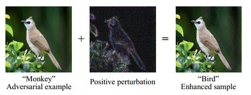
Adversarial examples have been shown to easily mislead neural networks, and many strategies have been proposed to defend them. To address the problem that most transformation-based defense strategies will degrade the accuracy of clean images, we proposed an Enhanced Image Transformation Generative Adversarial Network (EITGAN). Positive perturbations were employed in the EITGAN to counteract adversarial effects while enhancing the classified performance of the samples. We also used the image super-resolution method to mitigate the effect of adversarial perturbations. The proposed method does not require modification or retraining of the classifier. Extensive experiments demonstrated that the enhanced samples generated by the EITGAN effectively defended against adversarial attacks without compromising human visual recognition, and their classification performance was superior to that of clean images.
Citation: Junjie Zhao, Junfeng Wu, James Msughter Adeke, Guangjie Liu, Yuewei Dai. EITGAN: A Transformation-based Network for recovering adversarial examples[J]. Electronic Research Archive, 2023, 31(11): 6634-6656. doi: 10.3934/era.2023335
Adversarial examples have been shown to easily mislead neural networks, and many strategies have been proposed to defend them. To address the problem that most transformation-based defense strategies will degrade the accuracy of clean images, we proposed an Enhanced Image Transformation Generative Adversarial Network (EITGAN). Positive perturbations were employed in the EITGAN to counteract adversarial effects while enhancing the classified performance of the samples. We also used the image super-resolution method to mitigate the effect of adversarial perturbations. The proposed method does not require modification or retraining of the classifier. Extensive experiments demonstrated that the enhanced samples generated by the EITGAN effectively defended against adversarial attacks without compromising human visual recognition, and their classification performance was superior to that of clean images.

| [1] |
X. Li, J. Wu, Z. Sun, Z. Ma, J. Cao, J. Xue, Bsnet: Bi-similarity network for few-shot fine-grained image classification, IEEE Trans. Image Process., 30 (2021), 1318–1331. https://doi.org/10.1109/TIP.2020.3043128 doi: 10.1109/TIP.2020.3043128

|
| [2] | X. Chen, C. Xie, M. Tan, L. Zhang, C. J. Hsieh, B. Gong, Robust and accurate object detection via adversarial learning, in Proceedings of the IEEE/CVF Conference on Computer Vision and Pattern Recognition (CVPR), (2021), 16622–16631. |
| [3] | X. Li, H. He, X. Li, D. Li, G. Cheng, J. Shi, et al., Pointflow: Flowing semantics through points for aerial image segmentation, in Proceedings of the IEEE/CVF Conference on Computer Vision and Pattern Recognition (CVPR), (2021), 4217–4226. |
| [4] | A. Madry, A. Makelov, L. Schmidt, D. Tsipras, A. Vladu, Towards deep learning models resistant to adversarial attacks, in International Conference on Learning Representations, ICLR, (2018), 1–23. |
| [5] | P. Mangla, S. Jandial, S. Varshney, V. N. Balasubramanian, Advgan++: Harnessing latent layers for adversary generation, arXiv preprint, (2019), arXiv: 1908.00706. https://doi.org/10.48550/arXiv.1908.00706 |
| [6] | X. Li, L. Chen, J. Zhang, J. Larus, D. Wu, Watermarking-based defense against adversarial attacks on deep neural networks, in 2021 International Joint Conference on Neural Networks (IJCNN), IEEE, (2021), 1–8. https://doi.org/10.1109/IJCNN52387.2021.9534236 |
| [7] | Y. Zhu, X. Wei, Y. Zhu, Efficient adversarial defense without adversarial training: A batch normalization approach, in 2021 International Joint Conference on Neural Networks (IJCNN), IEEE, (2021), 1–8. https://doi.org/10.1109/IJCNN52387.2021.9533949 |
| [8] |
H. Kwon, Y. Kim, H. Yoon, D. Choi, Classification score approach for detecting adversarial example in deep neural network, Multimedia Tools Appl., 80 (2021), 10339–10360. https://doi.org/10.1007/s11042-020-09167-z doi: 10.1007/s11042-020-09167-z
|
| [9] | B. Huang, Z. Ke, Y. Wang, W. Wang, L. Shen, F. Liu, Adversarial defence by diversified simultaneous training of deep ensembles, in Proceedings of the AAAI Conference on Artificial Intelligence, AAAI, (2021), 7823–7831. https://doi.org/10.1609/aaai.v35i9.16955 |
| [10] | N. Das, M. Shanbhogue, S. T. Chen, F. Hohman, S. Li, L. Chen, et al., Shield: Fast, practical defense and vaccination for deep learning using jpeg compression, in Proceedings of the 24th ACM SIGKDD International Conference on Knowledge Discovery & Data Mining, Association for Computing Machinery, (2018), 196–204. |
| [11] | C. Xie, J. Wang, Z. Zhang, Z. Re, A. Yuille, Mitigating adversarial effects through randomization, in International Conference on Learning Representations, ICLR, (2018), 1–16. |
| [12] | C. Guo, M. Rana, M. Cisse, L. V. D. Maaten, Countering adversarial images using input transformations, in International Conference on Learning Representations, ICLR, (2018), 1–12. |
| [13] | A. Prakash, N. Moran, S. Garber, A. DiLillo, J. Storer, Deflecting adversarial attacks with pixel deflection, in Proceedings of the IEEE Conference on Computer Vision and Pattern Recognition (CVPR), (2018), 8571–8580. |
| [14] |
A. Mustafa, S. H. Khan, M. Hayat, J. Shen, L. Shao, Image super-resolution as a defense against adversarial attacks, IEEE Trans. Image Process., 29 (2020), 1711–1724. https://doi.org/10.1109/TIP.2019.2940533 doi: 10.1109/TIP.2019.2940533
|
| [15] |
R. K. Meleppat, K. E. Ronning, S. J. Karlen, M. E. Burns, E. N. Pugh, R. J. Zawadzki, In vivo multimodal retinal imaging of disease-related pigmentary changes in retinal pigment epithelium, Sci. Rep., 11 (2021), 16252. https://doi.org/10.1038/s41598-021-95320-z doi: 10.1038/s41598-021-95320-z
|
| [16] |
R. K. Meleppat, C. R. Fortenbach, Y. Jian, E. S. Martinez, K. Wagner, B. S. Modjtahedi, et al., In Vivo Imaging of Retinal and Choroidal Morphology and Vascular Plexuses of Vertebrates Using Swept-Source Optical Coherence Tomography, Transl. Vision Sci. Technol., 11 (2022), 11. https://doi.org/10.1167/tvst.11.8.11 doi: 10.1167/tvst.11.8.11
|
| [17] | K. M. Ratheesh, L. K. Seah, V. M. Murukeshan, Spectral phase-based automatic calibration scheme for swept source-based optical coherence tomography systems, Phys. Med. Biol., 61 (2016), 7652. |
| [18] | I. J. Goodfellow, J. Shlens, C. Szegedy, Explaining and harnessing adversarial examples, arXiv preprint, (2014), arXiv: 1412.6572. https://doi.org/10.48550/arXiv.1412.6572 |
| [19] | A. Kurakin, I. J. Goodfellow, S. Bengio, Adversarial examples in the physical world, in 5th International Conference on Learning Representations, ICLR, (2017), 1–14 |
| [20] | S. M. Moosavi-Dezfooli, A. Fawzi, P. Frossard, Deepfool: A simple and accurate method to fool deep neural networks, in Proceedings of the IEEE Conference on Computer Vision and Pattern Recognition, (2016), 2574–2582. |
| [21] | N. Carlini, D. Wagner, Towards evaluating the robustness of neural networks, in 2017 IEEE Symposium on Security and Privacy (sp), IEEE, (2017), 39–57. https://doi.org/10.1109/SP.2017.49 |
| [22] | Y. Luo, X. Boix, G. Roig, T. A. Poggio, Q. Zhao, Foveation-based mechanisms alleviate adversarial examples, arXiv preprint, (2015), arXiv: 1511.06292. https://doi.org/10.48550/arXiv.1511.06292 |
| [23] | B. Lim, S. Son, H. Kim, S. Nah, K. Mu Lee, Enhanced deep residual networks for single image super-resolution, in Proceedings of the IEEE Conference on Computer Vision and Pattern Recognition Workshops, (2017), 136–144. |
| [24] | W. Shi, J. Caballero, F. Huszár, J. Totz, A. P. Aitken, R. Bishop, et al., Real-time single image and video super-resolution using an efficient sub-pixel convolutional neural network, in Proceedings of the IEEE Conference on Computer Vision and Pattern Recognition, (2016), 1874–1883. |
| [25] | J. Deng, W. Dong, R. Socher, L. Li, K. Li, F. Li, Imagenet: A large-scale hierarchical image database, in 2009 IEEE Conference on Computer Vision and Pattern Recognition, IEEE, (2009), 248–255. https://doi.org/10.1109/CVPR.2009.5206848 |
| [26] | C. Szegedy, V. Vanhoucke, S. Ioffe, J. Shlens, Z. Wojna, Rethinking the inception architecture for computer vision, in 2016 IEEE Conference on Computer Vision and Pattern Recognition, IEEE, (2016), 2818–2826. https://doi.org/10.1109/CVPR.2016.308 |
| [27] | K. He, X. Zhang, S. Ren, J. Sun, Deep residual learning for image recognition, in 2016 IEEE Conference on Computer Vision and Pattern Recognition, IEEE, (2016), 770–778. https://doi.org/10.1109/CVPR.2016.90 |
| [28] | C. Szegedy, S. Ioffe, V. Vanhoucke, A. Alemi, Inception-v4, inception-resnet and the impact of residual connections on learning, in Proceedings of the AAAI Conference on Artificial Intelligence, AAAI, (2017), 4278–4284. https://doi.org/10.1609/aaai.v31i1.11231 |
| [29] | S. M. Moosavi-Dezfooli, A. Fawzi, O. Fawzi, P. Frossard, Universal adversarial perturbations, in Proceedings of the IEEE Conference on Computer Vision and Pattern Recognition, (2017), 1765–1773. |
| [30] |
N. Q. K. Le, Q. T. Ho, V. N. Nguyen, J. S. Chang, BERT-Promoter: An improved sequence-based predictor of DNA promoter using BERT pre-trained model and SHAP feature selection, Comput. Biol. Chem., 99 (2022), 107732. https://doi.org/10.1016/j.compbiolchem.2022.107732 doi: 10.1016/j.compbiolchem.2022.107732
|
| [31] |
N. Q. K. Le, T. T. Nguyen, Y. Y. Ou, Identifying the molecular functions of electron transport proteins using radial basis function networks and biochemical properties, J. Mol. Graphics Modell., 73 (2017), 166–178. https://doi.org/10.1016/j.jmgm.2017.01.003 doi: 10.1016/j.jmgm.2017.01.003
|
| [32] | S. Baluja, I. Fischer, Adversarial transformation networks: Learning to generate adversarial examples, arXiv preprint, (2017), arXiv: 1703.09387. https://doi.org/10.48550/arXiv.1703.09387 |
| [33] | C. Xiao, B. Li, J. Y. Zhu, W. He, M. Liu, D. Song, Generating adversarial examples with adversarial networks, arXiv preprint, (2018), arXiv: 1801.02610. https://doi.org/10.48550/arXiv.1801.02610 |
| [34] | B. Zhou, A. Khosla, A. Lapedriza, A. Oliva, A. Torralba, Learning deep features for discriminative localization, in 2016 IEEE Conference on Computer Vision and Pattern Recognition (CVPR), IEEE, (2016), 2921–2929. https://doi.org/10.1109/CVPR.2016.319 |
| [35] |
R. R. Selvaraju, M. Cogswell, A. Das, R. Vedantam, D. Parikh, D. Batra, Grad-cam: Visual explanations from deep networks via gradient-based localization, Int. J. Comput. Vision, 128 (2020), 336–359. https://doi.org/10.1007/s11263-019-01228-7 doi: 10.1007/s11263-019-01228-7
|
| [36] | D. Hendrycks, K. Zhao, S. Basart, J. Steinhardt, D. Song, Natural adversarial examples, in Proceedings of the IEEE/CVF Conference on Computer Vision and Pattern Recognition (CVPR), (2021), 15262–15271. |
| [37] | S. Zagoruyko, N. Komodakis, Wide residual networks, arXiv preprint, (2016), arXiv: 1605.07146. https://doi.org/10.48550/arXiv.1605.07146 |


Figures(7) / Tables(8)
Junjie Zhao, Junfeng Wu, James Msughter Adeke, Guangjie Liu, Yuewei Dai. EITGAN: A Transformation-based Network for recovering adversarial examples[J]. Electronic Research Archive, 2023, 31(11): 6634-6656. doi: 10.3934/era.2023335


 DownLoad: