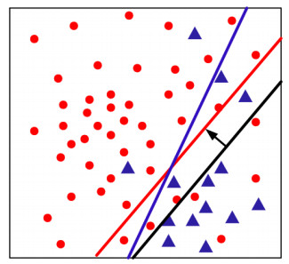
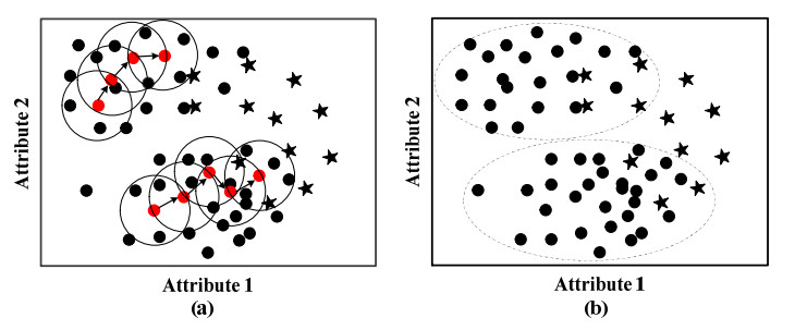
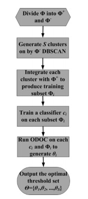
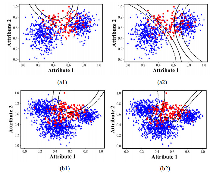
Class imbalance learning (CIL), which aims to addressing the performance degradation problem of traditional supervised learning algorithms in the scenarios of skewed data distribution, has become one of research hotspots in fields of machine learning, data mining, and artificial intelligence. As a postprocessing CIL technique, the decision threshold moving (DTM) has been verified to be an effective strategy to address class imbalance problem. However, no matter adopting random or optimal threshold designation ways, the classification hyperplane could be only moved parallelly, but fails to vary its orientation, thus its performance is restricted, especially on some complex and density variable data. To further improve the performance of the existing DTM strategies, we propose an improved algorithm called CDTM by dividing majority training instances into multiple different density regions, and further conducting DTM procedure on each region independently. Specifically, we adopt the well-known DBSCAN clustering algorithm to split training set as it could adapt density variation well. In context of support vector machine (SVM) and extreme learning machine (ELM), we respectively verified the effectiveness and superiority of the proposed CDTM algorithm. The experimental results on 40 benchmark class imbalance datasets indicate that the proposed CDTM algorithm is superior to several other state-of-the-art DTM algorithms in term of G-mean performance metric.
Citation: Mengke Lu, Shang Gao, Xibei Yang, Hualong Yu. Improving performance of decision threshold moving-based strategies by integrating density-based clustering technique[J]. Electronic Research Archive, 2023, 31(5): 2501-2518. doi: 10.3934/era.2023127
Class imbalance learning (CIL), which aims to addressing the performance degradation problem of traditional supervised learning algorithms in the scenarios of skewed data distribution, has become one of research hotspots in fields of machine learning, data mining, and artificial intelligence. As a postprocessing CIL technique, the decision threshold moving (DTM) has been verified to be an effective strategy to address class imbalance problem. However, no matter adopting random or optimal threshold designation ways, the classification hyperplane could be only moved parallelly, but fails to vary its orientation, thus its performance is restricted, especially on some complex and density variable data. To further improve the performance of the existing DTM strategies, we propose an improved algorithm called CDTM by dividing majority training instances into multiple different density regions, and further conducting DTM procedure on each region independently. Specifically, we adopt the well-known DBSCAN clustering algorithm to split training set as it could adapt density variation well. In context of support vector machine (SVM) and extreme learning machine (ELM), we respectively verified the effectiveness and superiority of the proposed CDTM algorithm. The experimental results on 40 benchmark class imbalance datasets indicate that the proposed CDTM algorithm is superior to several other state-of-the-art DTM algorithms in term of G-mean performance metric.

| [1] |
Y. C. Wang, C. H. Cheng, A multiple combined method for rebalancing medical data with class imbalances, Comput. Biol. Med., 134 (2021), 104527. https://doi.org/10.1016/j.compbiomed.2021.104527 doi: 10.1016/j.compbiomed.2021.104527

|
| [2] |
M. Zareapoor, P. Shamsolmoali, J. Yang, Oversampling adversarial network for class-imbalanced fault diagnosis, Mech. Syst. Signal Process., 149 (2021), 107175. https://doi.org/10.1016/j.ymssp.2020.107175 doi: 10.1016/j.ymssp.2020.107175
|
| [3] |
S. Fan, X. Zhang, Z. Song, Imbalanced sample selection with deep reinforcement learning for fault diagnosis, IEEE Trans. Ind. Inf., 18 (2021), 2518–2527. https://doi.org/10.1109/TⅡ.2021.3100284 doi: 10.1109/TⅡ.2021.3100284
|
| [4] |
N. Gupta, V. Jindal, P. Bedi, LIO-IDS: Handling class imbalance using LSTM and improved one-vs-one technique in intrusion detection system, Comput. Networks, 192 (2021), 108076. https://doi.org/10.1016/j.comnet.2021.108076 doi: 10.1016/j.comnet.2021.108076
|
| [5] |
Z. Li, M. Huang, G. Liu, C. Jiang, A hybrid method with dynamic weighted entropy for handling the problem of class imbalance with overlap in credit card fraud detection, Expert Syst. Appl., 175 (2021), 114750. https://doi.org/10.1016/j.eswa.2021.114750 doi: 10.1016/j.eswa.2021.114750
|
| [6] |
A. G. C. de Sá, A. C. M. Pereira, G. L. Pappa, A customized classification algorithm for credit card fraud detection, Eng. Appl. Artif. Intell., 72 (2018), 21–29. https://doi.org/10.1016/j.engappai.2018.03.011 doi: 10.1016/j.engappai.2018.03.011
|
| [7] |
B. Guo, C. Zhang, J. Liu, X. Ma, Improving text classification with weighted word embeddings via a multi-channel TextCNN model, Neurocomputing, 363 (2019), 366–374. https://doi.org/10.1016/j.neucom.2019.07.052 doi: 10.1016/j.neucom.2019.07.052
|
| [8] |
Y. Li, H. Guo, Q. Zhang, M. Gu, J. Yang, Imbalanced text sentiment classification using universal and domain-specific knowledge, Knowl. Based Syst., 160 (2018), 1–15. https://doi.org/10.1016/j.knosys.2018.06.019 doi: 10.1016/j.knosys.2018.06.019
|
| [9] |
L. Dou, F. Yang, L. Xu, Q. Zou, A comprehensive review of the imbalance classification of protein post-translational modifications, Briefings Bioinf., 22 (2021), bbab089. https://doi.org/10.1093/bib/bbab089 doi: 10.1093/bib/bbab089
|
| [10] |
M. Neyestani, F. Sarmadian, A. Jafari, A. Keshavarzi, A. Sharififar, Digital mapping of soil classes using spatial extrapolation with imbalanced data, Geoderma Reg., 26 (2021), e00422. https://doi.org/10.1016/j.geodrs.2021.e00422 doi: 10.1016/j.geodrs.2021.e00422
|
| [11] |
S. Ketu, P. K. Mishra, Scalable kernel-based SVM classification algorithm on imbalance air quality data for proficient healthcare, Complex Intell. Syst., 7 (2021), 2597–2615. https://doi.org/10.1007/s40747-021-00435-5 doi: 10.1007/s40747-021-00435-5
|
| [12] |
Y. S. Li, H. Chi, X. Y. Shao, M. L. Qi, B. G. Xu, A novel random forest approach for imbalance problem in crime linkage, Knowl. Based Syst., 195 (2020), 105738. https://doi.org/10.1016/j.knosys.2020.105738 doi: 10.1016/j.knosys.2020.105738
|
| [13] |
P. Soltanzadeh, M. Hashemzadeh, RCSMOTE: Range-Controlled synthetic minority over-sampling technique for handling the class imbalance problem, Inf. Sci, 542 (2021), 92–111. https://doi.org/10.1016/j.ins.2020.07.014 doi: 10.1016/j.ins.2020.07.014
|
| [14] |
S. Susan, A. Kumar, The balancing trick: optimized sampling of imbalanced datasets—a brief survey of the recent State of the Art, Eng. Rep., 3 (2021), e12298. https://doi.org/10.1002/eng2.12298 doi: 10.1002/eng2.12298
|
| [15] |
H. Guan, Y. Zhang, M. Xian, H. D. Cheng, X. Tang, SMOTE-WENN: Solving class imbalance and small sample problems by oversampling and distance scaling, Appl. Intell., 51 (2021), 1394–1409. https://doi.org/10.1007/s10489-020-01852-8 doi: 10.1007/s10489-020-01852-8
|
| [16] |
H. Yu, C. Sun, X. Yang, S. Zheng, H. Zou, Fuzzy support vector machine with relative density information for classifying imbalanced data, IEEE Trans. Fuzzy Syst., 27 (2019), 2353–2367. https://doi.org/10.1109/TFUZZ.2019.2898371 doi: 10.1109/TFUZZ.2019.2898371
|
| [17] |
H. Zhang, L. Jiang, C. Li, CS-ResNet: Cost-sensitive residual convolutional neural network for PCB cosmetic defect detection, Expert Syst. Appl., 185 (2021), 115673. https://doi.org/10.1016/j.eswa.2021.115673 doi: 10.1016/j.eswa.2021.115673
|
| [18] |
W. Pei, B. Xue, L. Shang, M. Zhang, Genetic programming for development of cost-sensitive classifiers for binary high-dimensional unbalanced classification, Appl. Soft Comput., 101 (2021), 106989. https://doi.org/10.1016/j.asoc.2020.106989 doi: 10.1016/j.asoc.2020.106989
|
| [19] |
Z. H. Zhou, X. Y. Liu, Training cost-sensitive neural networks with methods addressing the class imbalance problem, IEEE Trans. Knowl. Data Eng., 18 (2006), 63–77. https://doi.org/10.1109/TKDE.2006.17 doi: 10.1109/TKDE.2006.17
|
| [20] |
W. J. Lin, J. J. Chen, Class-imbalanced classifiers for high-dimensional data, Briefings Bioinf., 14 (2012), 13–26. https://doi.org/10.1093/bib/bbs006 doi: 10.1093/bib/bbs006
|
| [21] |
H. Yu, C. Mu, C. Sun, W. Yang, X. Yang, X. Zuo, Support vector machine-based optimized decision threshold adjustment strategy for classifying imbalanced data, Knowl. Based Syst., 76 (2015), 67–78. https://doi.org/10.1016/j.knosys.2014.12.007 doi: 10.1016/j.knosys.2014.12.007
|
| [22] |
H. Yu, C. Sun, X. Yang, W. Yang, J. Shen, Y. Qi, ODOC-ELM: Optimal decision outputs compensation-based extreme learning machine for classifying imbalanced data, Knowl. Based Syst., 92 (2016), 55–70. https://doi.org/10.1016/j.knosys.2015.10.012 doi: 10.1016/j.knosys.2015.10.012
|
| [23] |
K. Yang, Z. Yu, C. L. P. Chen, W. Cao, J. You, H. S. Wong, Incremental weighted ensemble broad learning system for imbalanced data, IEEE Trans. Knowl. Data Eng., 34 (2021), 5809–5824. https://doi.org/10.1109/TKDE.2021.3061428 doi: 10.1109/TKDE.2021.3061428
|
| [24] |
Z. Qi, Z. Zhang, A hybrid cost-sensitive ensemble for heart disease prediction, BMC Med. Inf. Decis. Making, 21 (2021), 1–18. https://doi.org/10.21203/rs.2.22946/v1 doi: 10.21203/rs.2.22946/v1
|
| [25] |
H. Du, Y. Zhang, K. Gang, L. Zhang, Y. C. Chen, Online ensemble learning algorithm for imbalanced data stream, Appl. Soft Comput., 107 (2021), 107378. https://doi.org/10.1016/j.asoc.2021.107378 doi: 10.1016/j.asoc.2021.107378
|
| [26] |
T. Hayashi, H. Fujita, One-class ensemble classifier for data imbalance problems, Appl. Intell., 52 (2022), 17073–17089. https://doi.org/10.1007/s10489-021-02671-1 doi: 10.1007/s10489-021-02671-1
|
| [27] |
E. Schubert, J. Sander, M. Ester, H. P. Kriegel, X. Xu, DBSCAN revisited, revisited: why and how you should (still) use DBSCAN, ACM Trans. Database Syst., 42 (2017), 1–21. https://doi.org/10.1145/3068335 doi: 10.1145/3068335
|
| [28] |
T. N. Tran, K. Drab, M. Daszykowski, Revised DBSCAN algorithm to cluster data with dense adjacent clusters, Chemom. Intell. Lab. Syst., 120 (2013), 92–96. https://doi.org/10.1016/j.chemolab.2012.11.006 doi: 10.1016/j.chemolab.2012.11.006
|
| [29] |
D. Birant, A. Kut, ST-DBSCAN: An algorithm for clustering spatial–temporal data, Data Knowl. Eng., 60 (2007), 208–221. https://doi.org/10.1016/j.datak.2006.01.013 doi: 10.1016/j.datak.2006.01.013
|
| [30] |
M. Ontivero-Ortega, A. Lage-Castellanos, G. Valente, R. Goebel, M. Valdes-Sosa, Fast Gaussian Naïve Bayes for searchlight classification analysis, Neuroimage, 163 (2017), 471–479. https://doi.org/10.1016/j.neuroimage.2017.09.001 doi: 10.1016/j.neuroimage.2017.09.001
|
| [31] |
R. D. Raizada, Y. S. Lee, Smoothness without smoothing: why Gaussian Naive Bayes is not naive for multi-subject searchlight studies, PloS One, 8 (2013), e69566. https://doi.org/10.1371/journal.pone.0069566 doi: 10.1371/journal.pone.0069566
|
| [32] |
W. S. Noble, What is a support vector machine? Nat. Biotechnol. , 24 (2006), 1565–1567. https://doi.org/10.1038/nbt1206-1565 doi: 10.1038/nbt1206-1565
|
| [33] |
C. C. Chang, C. J. Lin, LIBSVM: A library for support vector machines, ACM Trans. Intell. Syst. Technol., 2 (2011), 1–27. https://doi.org/10.1145/1961189.1961199 doi: 10.1145/1961189.1961199
|
| [34] |
G. B. Huang, Q. Y. Zhu, C. K. Siew, Extreme learning machine: theory and applications, Neurocomputing, 70 (2006), 489–501. https://doi.org/10.1016/j.neucom.2005.12.126 doi: 10.1016/j.neucom.2005.12.126
|
| [35] |
G. B. Huang, H. Zhou, X. Ding, R. Zhang, Extreme learning machine for regression and multiclass classification, IEEE Trans. Syst. Man Cybern. Part B Cybern., 42 (2011), 513–529. https://doi.org/10.1109/tsmcb.2011.2168604 doi: 10.1109/tsmcb.2011.2168604
|
| [36] |
H. Yu, J. Ni, S. Xu, B. Qin, H. Jv, Estimating harmfulness of class imbalance by scatter matrix based class separability measure, Intell. Data Anal., 18 (2014), 203–216. https://doi.org/10.3233/IDA-140637 doi: 10.3233/IDA-140637
|
| [37] | P. E. Gill, W. Murray, M. H. Wright, Practical Optimization, Academic Press, London, 1981. https://doi.org/10.2307/3616583 |
| [38] |
H. Guo, H. Liu, C. Wu, W. Zhi, Y. Xiao, W. She, Logistic discrimination based on G-mean and F-measure for imbalanced problem, J. Intell. Fuzzy Syst., 31 (2016), 1155–1166. https://doi.org/10.3233/ifs-162150 doi: 10.3233/ifs-162150
|
| [39] |
I. Triguero, S. González, J. M. Moyano, S. G. López, J. A. Fernández, J. L. Martín, KEEL 3.0: an open source software for multi-stage analysis in data mining, Int. J. Comput. Intell. Syst., 10 (2017), 1238–1249. https://doi.org/10.2991/ijcis.10.1.82 doi: 10.2991/ijcis.10.1.82
|
| [40] | J. Demšar, Statistical comparisons of classifiers over multiple data sets, J. Mach. Learn. Res., 7 (2006), 1–30. Available from: https://www.jmlr.org/papers/volume7/demsar06a/demsar06a.pdf. |
Figures(4) / Tables(8)
Mengke Lu, Shang Gao, Xibei Yang, Hualong Yu. Improving performance of decision threshold moving-based strategies by integrating density-based clustering technique[J]. Electronic Research Archive, 2023, 31(5): 2501-2518. doi: 10.3934/era.2023127


 DownLoad: