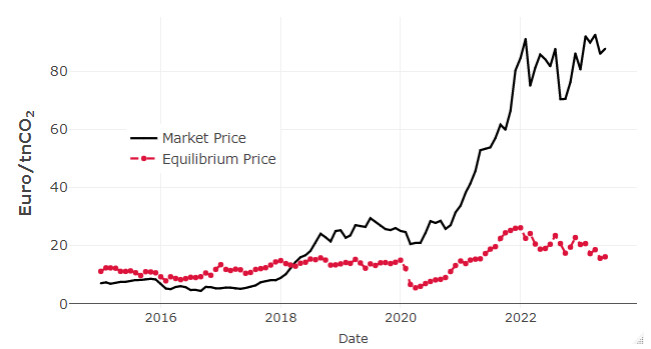
This study employed co-integration methodology to explore the fundamental drivers of carbon price in the European Union Emissions Trading System (EU ETS) during the transition from phase Ⅲ to phase Ⅳ, focusing on the interactions between the carbon market, energy sector, and macroeconomic factors. A novel approach of bilaterally modifying dummy variables was used to include the impact of regulatory event announcements on the EU carbon price. Long-term analysis revealed that coal prices exhibited a positive but statistically insignificant impact, while natural gas and oil prices show substantial and significant influences. Short-term dynamics indicated a self-adjusting mechanism, with gas and oil prices playing crucial roles. We found that the European stock market has a dampening effect on short-term carbon prices, whereas the commodity market exerted a counteractive force. In the energy sector, variations in European gas prices and shifts in nonrenewable electricity generation significantly influence short-term carbon price. Regulatory event announcements exhibited an overall negative and statistically significant trend. However, the relatively small magnitude of these coefficients underscored the modest impact of regulatory event announcements on short-term carbon prices within the EU ETS. Additionally, our study estimated the long-term equilibrium relationship between variables using ridge regression, serving as a proxy for the EU's equilibrium carbon price. We examined the disparities between this equilibrium and market prices. Two distinct phases emerged in the analysis. Before April 2018, the market price consistently lagged behind the equilibrium, suggesting an overestimation of the value of carbon emission rights. Subsequently, the market price consistently surpassed the equilibrium. In particular, the sharp increase in carbon prices from April to June 2020, driven by the COVID-19 pandemic, highlighted the sensitivity of the EU carbon market to external shocks.
Citation: Adnane Moulim, Sid'Ahmed Soumbara, Ahmed El Ghini. Cointegration analysis of fundamental drivers affecting carbon price dynamics in the EU ETS[J]. AIMS Environmental Science, 2025, 12(1): 165-192. doi: 10.3934/environsci.2025008
This study employed co-integration methodology to explore the fundamental drivers of carbon price in the European Union Emissions Trading System (EU ETS) during the transition from phase Ⅲ to phase Ⅳ, focusing on the interactions between the carbon market, energy sector, and macroeconomic factors. A novel approach of bilaterally modifying dummy variables was used to include the impact of regulatory event announcements on the EU carbon price. Long-term analysis revealed that coal prices exhibited a positive but statistically insignificant impact, while natural gas and oil prices show substantial and significant influences. Short-term dynamics indicated a self-adjusting mechanism, with gas and oil prices playing crucial roles. We found that the European stock market has a dampening effect on short-term carbon prices, whereas the commodity market exerted a counteractive force. In the energy sector, variations in European gas prices and shifts in nonrenewable electricity generation significantly influence short-term carbon price. Regulatory event announcements exhibited an overall negative and statistically significant trend. However, the relatively small magnitude of these coefficients underscored the modest impact of regulatory event announcements on short-term carbon prices within the EU ETS. Additionally, our study estimated the long-term equilibrium relationship between variables using ridge regression, serving as a proxy for the EU's equilibrium carbon price. We examined the disparities between this equilibrium and market prices. Two distinct phases emerged in the analysis. Before April 2018, the market price consistently lagged behind the equilibrium, suggesting an overestimation of the value of carbon emission rights. Subsequently, the market price consistently surpassed the equilibrium. In particular, the sharp increase in carbon prices from April to June 2020, driven by the COVID-19 pandemic, highlighted the sensitivity of the EU carbon market to external shocks.

| [1] | Schumpeter JA (1942) Capitalism, socialism and democracy, New York: Harper & Row, 36: 132–145. |
| [2] | Heine D, Semmler W, Mazzucato M, et al. (2019) Financing low-carbon transitions through carbon pricing and green bonds. Vierteljahrshefte Zur Wirtschaftsforschung 2: 29–49. |
| [3] |
Creti A, Nguyen DK (2015) Energy markets financialization, risk spillovers, and pricing models. Energ Policy 82: 260–263. https://doi.org/10.1016/j.enpol.2015.02.007 doi: 10.1016/j.enpol.2015.02.007

|
| [4] |
Amin A, Dogan E, Khan Z (2020) The impacts of different proxies for financialization on carbon emissions in top-ten emitter countries. Sci Total Environ 740: 140127–140127. https://doi.org/10.1016/j.scitotenv.2020.140127 doi: 10.1016/j.scitotenv.2020.140127
|
| [5] | Occhipinti Z, Verona R (2020) Kyoto protocol (kp). Climate Action 605–617. |
| [6] |
Alkathery MA, Chaudhuri K (2021) Co-movement between oil price, emission, renewable energy and energy equities: Evidence from GCC countries. J Environ Manage 297: 113350–113350. http://dx.doi.org/10.1016/j.jenvman.2021.113350 doi: 10.1016/j.jenvman.2021.113350
|
| [7] |
Boersen A, Scholtens B (2014) The relationship between European electricity markets and emission allowance futures prices in phase Ⅱ of the EU (European Union) emission trading scheme. Energy 74: 585–594. http://dx.doi.org/10.1016/j.energy.2014.07.024 doi: 10.1016/j.energy.2014.07.024
|
| [8] |
Carnero M, Olmo J, Pascual L (2018) Modelling the dynamics of fuel and EU allowance prices during phase 3 of the EU ETS. Energies 11: 3148–3148. http://dx.doi.org/10.3390/en11113148 doi: 10.3390/en11113148
|
| [9] |
Chang K, Zhang C, Wang HW (2020) Asymmetric dependence structures between emission allowances and energy markets: New evidence from China's emissions trading scheme pilots. Environ Sci Pollut R 27: 21140–21158. http://dx.doi.org/10.1007/s11356-020-08237-x doi: 10.1007/s11356-020-08237-x
|
| [10] |
Chevallier J (2012) Time-varying correlations in oil, gas and CO2 prices: An application using BEKK, CCC and DCC-MGARCH models. Appl. Econ 44: 4257–4274. http://dx.doi.org/10.1080/00036846.2011.589809 doi: 10.1080/00036846.2011.589809
|
| [11] |
Alberola E, Chevallier J, Chèze B (2008) Price drivers and structural breaks in European carbon prices 2005–2007. Energ Policy 36: 787–797. http://dx.doi.org/10.1016/j.enpol.2007.10.029 doi: 10.1016/j.enpol.2007.10.029
|
| [12] |
Tan XP, Wang XY (2017) Dependence changes between the carbon price and its fundamentals: A quantile regression approach. Appl Energ 190: 306–325. http://dx.doi.org/10.1016/j.apenergy.2016.12.116 doi: 10.1016/j.apenergy.2016.12.116
|
| [13] |
Tan X, Sirichand K, Vivian A, et al. (2020) How connected is the carbon market to energy and financial markets? A systematic analysis of spillovers and dynamics. Energ Econ 90: 104870–104870. http://dx.doi.org/10.1016/j.eneco.2020.104870 doi: 10.1016/j.eneco.2020.104870
|
| [14] |
Wang ZJ, Zhao LT (2021) The impact of the global stock and energy market on EU ETS: A structural equation modelling approach. J Clean Prod 289: 125140–125140. http://dx.doi.org/10.1016/j.jclepro.2020.125140 doi: 10.1016/j.jclepro.2020.125140
|
| [15] |
Paolella MS, Taschini L (2008) An econometric analysis of emission allowance prices. J Bank Financ 32: 2022–2032. http://dx.doi.org/10.1016/j.jbankfin.2007.09.024 doi: 10.1016/j.jbankfin.2007.09.024
|
| [16] | Benz E, Trück S (2009) Modeling the price dynamics of CO2 emission allowances. Energ Econ 31: 4–15. |
| [17] | Daskalakis G, Psychoyios D, Markellos RN (2009) Modeling CO2 emission allowance prices and derivatives: Evidence from the European trading scheme. J Bank Financ 33: 1230–1241. |
| [18] | Chevallier J, Nguyen DK, Reboredo JC (2019) A conditional dependence approach to CO2-energy price relationships. Energ Econ 81: 812–821. |
| [19] | Rodríguez RJ (2019) What happens to the relationship between EU allowances prices and stock market indices in Europe? Energ Econ 81: 13–24. http://dx.doi.org/10.1016/j.eneco.2019.03.002 |
| [20] |
Zhao LT, Miao J, Qu S, et al. (2021) A multi-factor integrated model for carbon price forecasting: Market interaction promoting carbon emission reduction. Sci Total Environ 796: 149110–149110. http://dx.doi.org/10.1016/j.scitotenv.2021.149110 doi: 10.1016/j.scitotenv.2021.149110
|
| [21] | Creti A, Jouvet PA, Mignon V (2012) Carbon price drivers: Phase Ⅰ versus Phase Ⅱ equilibrium? Energ Econ 34: 327–334. http://dx.doi.org/10.1016/j.eneco.2011.11.001 |
| [22] |
Hammoudeh S, Nguyen DK, Sousa RM (2014) Energy prices and CO2 emission allowance prices: A quantile regression approach. Energ Policy 70: 201–206. http://dx.doi.org/10.1016/j.enpol.2014.02.017 doi: 10.1016/j.enpol.2014.02.017
|
| [23] | Hammoudeh S, Nguyen DK, Sousa RM (2014) What explain the short-term dynamics of the prices of CO2 emissions? Energ Econ 46: 122–135. http://dx.doi.org/10.1016/j.eneco.2014.09.003 |
| [24] |
Zhao X, Han M, Ding L, et al. (2018) Usefulness of economic and energy data at different frequencies for carbon price forecasting in the EU ETS. Appl Energ 216: 132–141. http://dx.doi.org/10.1016/j.apenergy.2018.02.003 doi: 10.1016/j.apenergy.2018.02.003
|
| [25] |
Adekoya OB, Oliyide JA, Noman A (2021) The volatility connectedness of the EU carbon market with commodity and financial markets in time- and frequency-domain: The role of the U.S. economic policy uncertainty. Resour Policy 74: 102252–102252. http://dx.doi.org/10.1016/j.resourpol.2021.102252 doi: 10.1016/j.resourpol.2021.102252
|
| [26] |
Wu Y, Zhang C, Yun P, et al. (2021) Time-frequency analysis of the interaction mechanism between European carbon and crude oil markets. Energy Environ 32: 1331–1357. http://dx.doi.org/10.1177/0958305x211002457 doi: 10.1177/0958305x211002457
|
| [27] |
Yuan N, Yang L (2020) Asymmetric risk spillover between financial market uncertainty and the carbon market: A GAS-DCS-copula approach. J Clean Prod 259: 120750–120750. http://dx.doi.org/10.1016/j.jclepro.2020.120750 doi: 10.1016/j.jclepro.2020.120750
|
| [28] | Bataller MM, Pardo A, Valor E (2007) CO2 prices, energy and weather. Energy J 28. http://dx.doi.org/10.5547/issn0195-6574-ej-vol28-no3-5 |
| [29] |
Zhang YJ, Sun YF (2016) The dynamic volatility spillover between European carbon trading market and fossil energy market. J Clean Prod 112: 2654–2663. http://dx.doi.org/10.1016/j.jclepro.2015.09.118 doi: 10.1016/j.jclepro.2015.09.118
|
| [30] | Dou Y, Li Y, Dong K, et al. (2022) Dynamic linkages between economic policy uncertainty and the carbon futures market: Does Covid-19 pandemic matter? Resour Policy 75: 102455–102455. http://dx.doi.org/10.1016/j.resourpol.2021.102455 |
| [31] |
Wang Y, Guo Z (2018) The dynamic spillover between carbon and energy markets: New evidence. Energy 149: 24–33. http://dx.doi.org/10.1016/j.energy.2018.01.145 doi: 10.1016/j.energy.2018.01.145
|
| [32] |
Gong X, Shi R, Xu J, et al. (2021) Analyzing spillover effects between carbon and fossil energy markets from a time-varying perspective. Appl Energ 285: 116384–116384. http://dx.doi.org/10.1016/j.apenergy.2020.116384 doi: 10.1016/j.apenergy.2020.116384
|
| [33] |
Hintermann B. (2010) Allowance price drivers in the first phase of the EU ETS. J Environ Econ Manag 59: 43–56. http://dx.doi.org/10.1016/j.jeem.2009.07.002 doi: 10.1016/j.jeem.2009.07.002
|
| [34] |
Lovcha Y, Laborda AP, Sikor I (2022) The determinants of CO2 prices in the EU emission trading system. Appl Energ 305: 117903–117903. http://dx.doi.org/10.1016/j.apenergy.2021.117903 doi: 10.1016/j.apenergy.2021.117903
|
| [35] | Levinson A. (2010) Belts and suspenders: Interactions among climate policy regulations. Nation Bureau Econo Res. http://dx.doi.org/10.3386/w16109 |
| [36] | Gillum L (2013) Markets for pollution allowances: What are the (new) lessons? CFA Digest 43. http://dx.doi.org/10.2469/dig.v43.n3.7 |
| [37] | Kossoy A, Guigon P (2012) State and trends of the carbon market 2012, World Bank, Washington, DC. Available from: http://hdl.handle.net/10986/13336. |
| [38] |
Rittler D (2011) Price discovery and volatility spillovers in the European Union emissions trading scheme: A high-frequency analysis. J Bank Financ 36: 774–785. https://doi.org/10.1016/j.jbankfin.2011.09.009 doi: 10.1016/j.jbankfin.2011.09.009
|
| [39] |
Koch N, Grosjean G, Fuss S, et al. (2015) Politics matters: Regulatory events as catalysts for price formation under cap-and-trade. J Environ Econ Manag 78: 121–139. https://doi.org/10.1016/j.jeem.2016.03.004 doi: 10.1016/j.jeem.2016.03.004
|
| [40] |
Chevallier J (2009) Carbon futures and macroeconomic risk factors: A view from the EU ETS. Energ Econ 31: 614–625. http://dx.doi.org/10.1016/j.eneco.2009.02.008 doi: 10.1016/j.eneco.2009.02.008
|
| [41] |
Lutz BJ, Pigorsch U, Rotfuss W (2013) Nonlinearity in cap-and-trade systems: The EUA price and its fundamentals. Energ Econ 40: 222–232. https://doi.org/10.1016/j.eneco.2013.05.022 doi: 10.1016/j.eneco.2013.05.022
|
| [42] |
Schmidbauer H, Rösch A (2012) OPEC news announcements: Effects on oil price expectation and volatility. Energ Econ 34: 1656–1663. http://dx.doi.org/10.1016/j.eneco.2012.01.006 doi: 10.1016/j.eneco.2012.01.006
|
| [43] |
Jia JJ, Xu JH, Fan Y (2016) The impact of verified emissions announcements on the European Union emissions trading scheme: A bilaterally modified dummy variable modelling analysis. Appl Energy 173: 567–577. http://dx.doi.org/10.1016/j.apenergy.2016.04.027 doi: 10.1016/j.apenergy.2016.04.027
|
| [44] |
Jia J, Wu H, Zhu X, et al. (2019) Price break points and impact process evaluation in the EU ETS. Emerg Mark Financ Tr 56: 1691–1714. http://dx.doi.org/10.1080/1540496x.2019.1694888 doi: 10.1080/1540496x.2019.1694888
|
| [45] | Känzig D (2023) The unequal economic consequences of carbon pricing. Nation Bureau Econ Res. http://dx.doi.org/10.3386/w31221 |
| [46] | European commission. (2023) Climate Action News. Available from: https://climate.ec.europa.eu/news-your-voice/news-en. |
| [47] |
Tian W (2013) A review of sensitivity analysis methods in building energy analysis. Renew Sust Energ Rev 20: 411–419. http://dx.doi.org/10.1016/j.rser.2012.12.014 doi: 10.1016/j.rser.2012.12.014
|
| [48] |
Li L, Lu Z (2013) Importance analysis for models with correlated variables and its sparse grid solution. Reliab Eng Syst Safe 119: 207–217. http://dx.doi.org/10.1016/j.ress.2013.06.036 doi: 10.1016/j.ress.2013.06.036
|
| [49] |
Grömping U (2015) Variable importance in regression models. WIREs Comput Stat 7: 137–152. http://dx.doi.org/10.1002/wics.1346 doi: 10.1002/wics.1346
|
| [50] |
Bi J (2012) A review of statistical methods for determination of relative importance of correlated predictors and identification of drivers of consumer liking. J Sens Stud 27: 87–101. http://dx.doi.org/10.1111/j.1745-459x.2012.00370.x doi: 10.1111/j.1745-459x.2012.00370.x
|
| [51] | Zuber V, Strimmer K (2011) High-dimensional regression and variable selection using CAR scores. Stat Appl Genet Mol 10. http://dx.doi.org/10.2202/1544-6115.1730 |
| [52] |
Grömping U (2006) Relative importance for linear regression in R: The package relaimpo. J Stat Softw 17: 1–27. http://dx.doi.org/10.18637/jss.v017.i01 doi: 10.18637/jss.v017.i01
|
| [53] | Pesaran MH, Pesaran B (1997) Working with Microfit 4.0: Interactive econometric analysis, Oxford University Press. |
| [54] |
Pesaran MH, Shin Y, Smith RJ (2001) Bounds testing approaches to the analysis of level relationships. J Appl Econ 16: 289–326. http://dx.doi.org/10.1002/jae.616 doi: 10.1002/jae.616
|
| [55] |
Engle RF, Granger CWJ (1987) Co-integration and error correction: Representation, estimation, and testing. Econometrica 55: 251–276. http://dx.doi.org/10.2307/1913236 doi: 10.2307/1913236
|
| [56] |
Hoerl AE, Kennard RW (1970) Ridge regression: Applications to nonorthogonal problems. Technometrics 12: 69–82. http://dx.doi.org/10.1080/00401706.1970.10488635 doi: 10.1080/00401706.1970.10488635
|
| [57] |
Dickey DA, Fuller WA (1981) Likelihood ratio statistics for autoregressive time series with a unit root. Econometrica 49: 1057. http://dx.doi.org/10.2307/1912517 doi: 10.2307/1912517
|
| [58] |
Perron P, Phillips PCB (1987) Does GNP have a unit root?: A re-evaluation. Econ Lett 23: 139–145. http://dx.doi.org/10.1016/0165-1765(87)90027-9 doi: 10.1016/0165-1765(87)90027-9
|
| [59] |
Aatola P, Ollikainen M, Toppinen A (2013) Price determination in the EU ETS market: Theory and econometric analysis with market fundamentals. Energ Econ 36: 380–395. http://dx.doi.org/10.1016/j.eneco.2012.09.009 doi: 10.1016/j.eneco.2012.09.009
|
| [60] |
Zhu B, Ye S, Han D, et al. (2019) A multiscale analysis for carbon price drivers. Energ Econo 78: 202–216. http://dx.doi.org/10.1016/j.eneco.2018.11.007 doi: 10.1016/j.eneco.2018.11.007
|
| [61] |
Duan K, Ren X, Shi Y, et al. (2021) The marginal impacts of energy prices on carbon price variations: Evidence from a quantile-on-quantile approach. Energ Econ 95: 105131–105131. http://dx.doi.org/10.1016/j.eneco.2021.105131 doi: 10.1016/j.eneco.2021.105131
|
| [62] |
Brown RL, Durbin J, Evans JM (1975) Techniques for testing the constancy of regression relationships over time. J Roy Stat Soc B 37: 149–163. http://dx.doi.org/10.1111/j.2517-6161.1975.tb01532.x doi: 10.1111/j.2517-6161.1975.tb01532.x
|
| [63] |
Fang D, Yu B (2021) Driving mechanism and decoupling effect of PM$_{2.5}$ emissions: Empirical evidence from China's industrial sector. Energ Policy 149: 112017–112017. http://dx.doi.org/10.1016/j.enpol.2020.112017 doi: 10.1016/j.enpol.2020.112017
|
| [64] |
Semmler W, Lessmann K, Tahri I, et al. (2022) Green transition, investment horizon, and dynamic portfolio decisions. Ann Oper Res 334: 265–286. http://dx.doi.org/10.1007/s10479-022-05018-2 doi: 10.1007/s10479-022-05018-2
|
| [65] |
Hu J, Graus WC, Lam L, et al. (2015) Ex-ante evaluation of EU ETS during 2013–2030: EU-internal abatement. Energ Policy 77: 152–163. http://dx.doi.org/10.1016/j.enpol.2014.11.023 doi: 10.1016/j.enpol.2014.11.023
|
| [66] |
Bocse AM (2019) The UK's decision to leave the European Union (Brexit) and its impact on the EU as a climate change actor. Clim Policy 20: 265–274. http://dx.doi.org/10.1080/14693062.2019.1701402 doi: 10.1080/14693062.2019.1701402
|
| [67] |
Ye J, Xue M (2021) Influences of sentiment from news articles on EU carbon prices. Energ Econ 101: 105393–105393. http://dx.doi.org/10.1016/j.eneco.2021.105393 doi: 10.1016/j.eneco.2021.105393
|
| [68] |
Low S, Boettcher M (2020) Delaying decarbonization: Climate governmentalities and sociotechnical strategies from Copenhagen to Paris. Earth Syst Gov 5: 100073–100073. http://dx.doi.org/10.1016/j.esg.2020.100073 doi: 10.1016/j.esg.2020.100073
|
| [69] | Gerlagh R, Heijmans RJRK, Rosendahl KE (2022) Shifting concerns for the EU ETS: Are carbon prices becoming too high? Environ Res Lett 17: 054018–054018. http://dx.doi.org/10.1088/1748-9326/ac63d6 |
| [70] |
Beck U, Andersen PK (2020) Endogenizing the cap in a cap-and-trade system: Assessing the agreement on EU ETS phase 4. Environ Resource Econ 77: 781–811. http://dx.doi.org/10.1007/s10640-020-00518-w doi: 10.1007/s10640-020-00518-w
|
| [71] |
Rubio EV, Morales MDH, Valdivieso FG (2023) Using EGARCH models to predict volatility in unconsolidated financial markets: The case of European carbon allowances. J Environ Stud Sci 13: 500–509. http://dx.doi.org/10.1007/s13412-023-00838-5 doi: 10.1007/s13412-023-00838-5
|
| [72] |
Haxhimusa A, Liebensteiner M (2021) Effects of electricity demand reductions under a carbon pricing regime on emissions: Lessons from COVID-19. Energ Policy 156: 112392–112392. http://dx.doi.org/10.1016/j.enpol.2021.112392 doi: 10.1016/j.enpol.2021.112392
|
| [73] |
Dong H, Tan X, Cheng S, et al. (2022) COVID-19, recovery policies and the resilience of EU ETS. Econ Chang Restruct 56: 2965–2991. http://dx.doi.org/10.1007/s10644-021-09372-2 doi: 10.1007/s10644-021-09372-2
|
Figures(5) / Tables(9)

Adnane Moulim, Sid'Ahmed Soumbara, Ahmed El Ghini. Cointegration analysis of fundamental drivers affecting carbon price dynamics in the EU ETS[J]. AIMS Environmental Science, 2025, 12(1): 165-192. doi: 10.3934/environsci.2025008


 DownLoad: