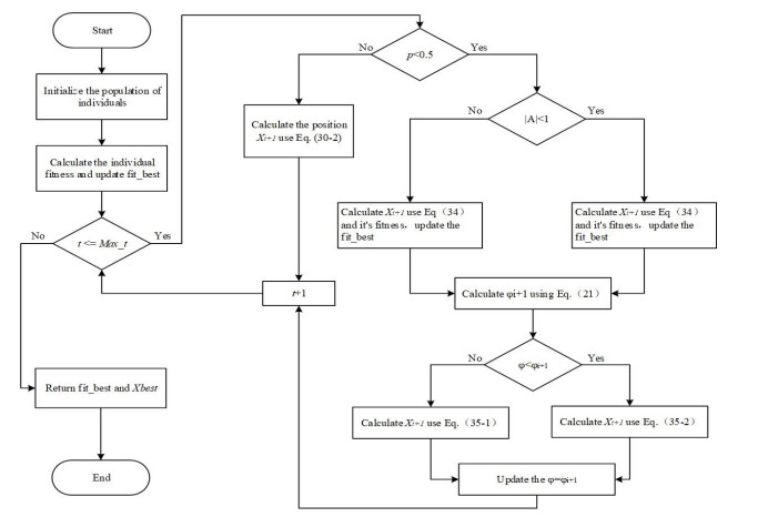
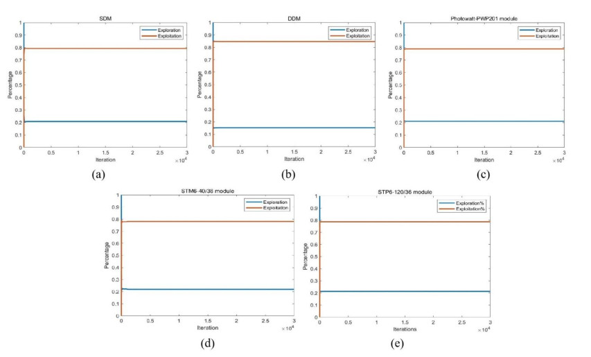
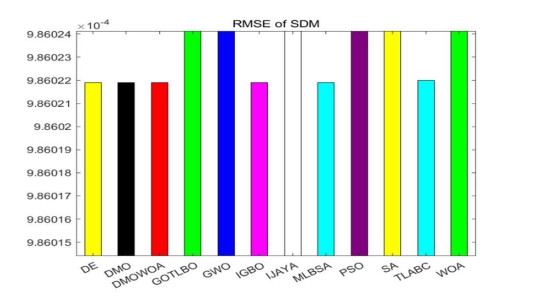
This article proposed adaptive hybrid dwarf mongoose optimization (DMO) with whale optimization algorithm (DMOWOA) to extract solar cell model parameters. In DMOWOA, the whale optimization algorithm (WOA) is used to enhance the capability of DMO in escaping local optima, while introducing inertial weights to achieve a balance between exploration and exploitation. The DMOWOA performances are tested through the solving of the single diode model, double diode model, and photovoltaic (PV) modules. Finally, the DMOWOA is compared with six well-known algorithms and other optimization methods. The experimental results demonstrate that the proposed DMOWOA exhibits remarkable competitiveness in convergence speed, robustness, and accuracy.
Citation: Shijian Chen, Yongquan Zhou, Qifang Luo. Hybrid adaptive dwarf mongoose optimization with whale optimization algorithm for extracting photovoltaic parameters[J]. AIMS Energy, 2024, 12(1): 84-118. doi: 10.3934/energy.2024005
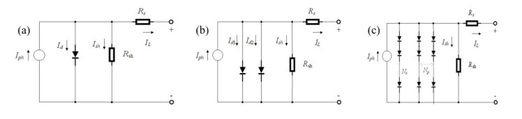
This article proposed adaptive hybrid dwarf mongoose optimization (DMO) with whale optimization algorithm (DMOWOA) to extract solar cell model parameters. In DMOWOA, the whale optimization algorithm (WOA) is used to enhance the capability of DMO in escaping local optima, while introducing inertial weights to achieve a balance between exploration and exploitation. The DMOWOA performances are tested through the solving of the single diode model, double diode model, and photovoltaic (PV) modules. Finally, the DMOWOA is compared with six well-known algorithms and other optimization methods. The experimental results demonstrate that the proposed DMOWOA exhibits remarkable competitiveness in convergence speed, robustness, and accuracy.

| [1] |
Shindell D, Smith CJ (2019) Climate and air-quality benefits of a realistic phase-out of fossil fuels. Nature 573: 408–411. https://doi.org/10.1038/s41586-019-1554-z doi: 10.1038/s41586-019-1554-z

|
| [2] |
Hu G, Wang J, Su Z, et al. (2019) Performance evaluation of twin piezoelectric wind energy harvesters under mutual interference. Appl Phys Lett 115: 073901. https://doi.org/10.1063/1.5109457 doi: 10.1063/1.5109457
|
| [3] |
Cabrera P, Carta JA, Lund H, et al. (2021) Large-scale optimal integration of wind and solar photovoltaic power in water-energy systems on islands. Energy Convers Manage 235: 113982. https://doi.org/10.1016/j.enconman.2021.113982 doi: 10.1016/j.enconman.2021.113982
|
| [4] |
Askarzadeh A, Rezazadeh A (2013) Artificial bee swarm optimization algorithm for parameters identification of solar cell models. Appl Energy 102: 943–949. https://doi.org/10.1016/j.apenergy.2012.09.052 doi: 10.1016/j.apenergy.2012.09.052
|
| [5] |
Jordehi AR (2018) Enhanced leader particle swarm optimisation (ELPSO): An efficient algorithm for parameter estimation of photovoltaic (PV) cells and modules. Sol Energy 159: 78–87. https://doi.org/10.1016/j.solener.2017.10.063 doi: 10.1016/j.solener.2017.10.063
|
| [6] |
Alam DF, Yousri DA, Eteiba MB (2015) Flower pollination algorithm based solar PV parameter estimation. Energy Convers Manage 101: 410–422. https://doi.org/10.1016/j.enconman.2015.05.074 doi: 10.1016/j.enconman.2015.05.074
|
| [7] |
Humada AM, Hojabri M, Mekhilef S, et al (2016) Solar cell parameters extraction based on single and double-diode models: A review. Renewable Sustainable Energy Rev 56: 494–509. https://doi.org/10.1016/j.rser.2015.11.051 doi: 10.1016/j.rser.2015.11.051
|
| [8] |
Chin VJ, Salam Z, Ishaque K (2015) Cell modelling and model parameters estimation techniques for photovoltaic simulator application: A review. Appl Energy 154: 500–519. https://doi.org/10.1016/j.apenergy.2015.05.035 doi: 10.1016/j.apenergy.2015.05.035
|
| [9] |
Li S, Gong W, Gu Q (2021) A comprehensive survey on meta-heuristic algorithms for parameter extraction of photovoltaic models. Renewable Sustainable Energy Rev 141: 110828. https://doi.org/10.1016/j.rser.2021.110828 doi: 10.1016/j.rser.2021.110828
|
| [10] |
Chan DSH, Phang JCH (1987) Analytical methods for the extraction of solar-cell single-and double-diode model parameters from Ⅳ characteristics. IEEE Trans Electron Devices 34: 286–293. https://doi.org/10.1109/T-ED.1987.22920 doi: 10.1109/T-ED.1987.22920
|
| [11] |
Adeel M, Hassan AK, Sher HA, et al. (2021) A grade point average assessment of analytical and numerical methods for parameter extraction of a practical PV device. Renewable Sustainable Energy Rev 142: 110826. https://doi.org/10.1016/j.rser.2021.110826 doi: 10.1016/j.rser.2021.110826
|
| [12] |
Easwarakhanthan T, Bottin J, Bouhouch I, et al. (1986) Nonlinear minimization algorithm for determining the solar cell parameters with microcomputers. Int J Sol Energy 4: 1–12. https://doi.org/10.1080/01425918608909835 doi: 10.1080/01425918608909835
|
| [13] |
Nassar-Eddine I, Obbadi A, Errami Y, et al. (2016) Parameter estimation of photovoltaic modules using iterative method and the Lambert W function: A comparative study. Energy Convers Manage 119: 37–48. https://doi.org/10.1016/j.enconman.2016.04.030 doi: 10.1016/j.enconman.2016.04.030
|
| [14] |
Et-Torabi K, Nassar-Eddine I, Obbadi A, et al. (2017) Parameters estimation of the single and double diode photovoltaic models using a Gauss-Seidel algorithm and analytical method: A comparative study. Energy Convers Manage 148: 1041–1054. https://doi.org/10.1016/j.enconman.2017.06.064 doi: 10.1016/j.enconman.2017.06.064
|
| [15] |
Chan DSH, Phillips JR, Phang JCH (1986) A comparative study of extraction methods for solar cell model parameters. Solid-State Electron 29: 329–337. https://doi.org/10.1016/0038-1101(86)90212-1 doi: 10.1016/0038-1101(86)90212-1
|
| [16] |
Gao S, Yu Y, Wang Y, et al. (2019) Chaotic local search-based differential evolution algorithms for optimization. IEEE Trans Syst Man Cybern: Syst 51: 3954–3967. https://doi.org/10.1109/TSMC.2019.2956121 doi: 10.1109/TSMC.2019.2956121
|
| [17] |
Hansen N, Müller SD, Koumoutsakos P (2003) Reducing the time complexity of the derandomized evolution strategy with covariance matrix adaptation (CMA-ES). J Evol Comput 11: 1–18. https://doi.org/10.1162/106365603321828970 doi: 10.1162/106365603321828970
|
| [18] |
Guzman R, Oliveira R, Ramos F (2020) Heteroscedastic bayesian optimisation for stochastic model predictive control. IEEE Rob Autom Lett 6: 56–63. https://doi.org/10.1109/LRA.2020.3028830 doi: 10.1109/LRA.2020.3028830
|
| [19] |
Zagrouba M, Sellami A, Bouaïcha M, et al. (2010) Identification of PV solar cells and modules parameters using the genetic algorithms: Application to maximum power extraction. Sol Energy 84: 860–866. https://doi.org/10.1016/j.solener.2010.02.012 doi: 10.1016/j.solener.2010.02.012
|
| [20] |
Hu Z, Gong W, Li S (2021) Reinforcement learning-based differential evolution for parameters extraction of photovoltaic models. Energy Rep 7: 916–928. https://doi.org/10.1016/j.egyr.2021.01.096 doi: 10.1016/j.egyr.2021.01.096
|
| [21] |
Ye M, Wang X, Xu Y (2009) Parameter extraction of solar cells using particle swarm optimization. J Appl Phys 105: 094502. https://doi.org/10.1063/1.3122082 doi: 10.1063/1.3122082
|
| [22] |
El-Naggar KM, AlRashidi MR, AlHajri MF, et al. (2012) Simulated annealing algorithm for photovoltaic parameters identification. Sol Energy 86: 266–274. https://doi.org/10.1016/j.solener.2011.09.032 doi: 10.1016/j.solener.2011.09.032
|
| [23] |
Allam D, Yousri DA, Eteiba MB (2016) Parameters extraction of the three diode model for the multi-crystalline solar cell/module using Moth-Flame Optimization Algorithm. Energy Convers Manage 123: 535–548. https://doi.org/10.1016/j.enconman.2016.06.052 doi: 10.1016/j.enconman.2016.06.052
|
| [24] |
Oliva D, Cuevas E, Pajares G (2014) Parameter identification of solar cells using artificial bee colony optimization. Energy 72: 93–102. https://doi.org/10.1016/j.energy.2014.05.011 doi: 10.1016/j.energy.2014.05.011
|
| [25] |
Yu K, Chen X, Wang X, et al. (2017) Parameters identification of photovoltaic models using self-adaptive teaching-learning-based optimization. Energy Convers Manage 145: 233–246. https://doi.org/10.1016/j.enconman.2017.04.054 doi: 10.1016/j.enconman.2017.04.054
|
| [26] |
Zhang Y, Ma M, Jin Z (2020) Comprehensive learning Jaya algorithm for parameter extraction of photovoltaic models. Energy 211: 118644. https://doi.org/10.1016/j.energy.2020.118644 doi: 10.1016/j.energy.2020.118644
|
| [27] |
Li S, Gu Q, Gong W, et al. (2020) An enhanced adaptive differential evolution algorithm for parameter extraction of photovoltaic models. Energy Convers Manage 205: 112443. https://doi.org/10.1016/j.enconman.2019.112443 doi: 10.1016/j.enconman.2019.112443
|
| [28] |
Merchaoui M, Sakly A, Mimouni MF (2018) Particle swarm optimisation with adaptive mutation strategy for photovoltaic solar cell/module parameter extraction. Energy Convers Manage 175: 151–163. https://doi.org/10.1016/j.enconman.2018.08.081 doi: 10.1016/j.enconman.2018.08.081
|
| [29] |
Ishaque K, Salam Z (2011) An improved modeling method to determine the model parameters of photovoltaic (PV) modules using differential evolution (DE). Sol Energy 85: 2349–2359. https://doi.org/10.1016/j.solener.2011.06.025 doi: 10.1016/j.solener.2011.06.025
|
| [30] |
Xiong G, Zhang J, Yuan X, et al. (2018) Parameter extraction of solar photovoltaic models by means of a hybrid differential evolution with whale optimization algorithm. Sol Energy 176: 742–761. https://doi.org/10.1016/j.solener.2018.10.050 doi: 10.1016/j.solener.2018.10.050
|
| [31] |
Jiang LL, Maskell DL, Patra JC (2013) Parameter estimation of solar cells and modules using an improved adaptive differential evolution algorithm. Appl Energy 112: 185–193. https://doi.org/10.1016/j.apenergy.2013.06.004 doi: 10.1016/j.apenergy.2013.06.004
|
| [32] |
Chen X, Xu B, Mei C, et al. (2018) Teaching-learning-based artificial bee colony for solar photovoltaic parameter estimation. Appl Energy 212: 1578–1588. https://doi.org/10.1016/j.apenergy.2017.12.115 doi: 10.1016/j.apenergy.2017.12.115
|
| [33] |
Niu Q, Zhang H, Li K (2014) An improved TLBO with elite strategy for parameters identification of PEM fuel cell and solar cell models. Int J Hydrogen Energy 39: 3837–3854. https://doi.org/10.1016/j.ijhydene.2013.12.110 doi: 10.1016/j.ijhydene.2013.12.110
|
| [34] |
Chen X, Yu K, Du W, et al. (2016) Parameters identification of solar cell models using generalized oppositional teaching learning based optimization. Energy 99: 170–180. https://doi.org/10.1016/j.energy.2016.01.052 doi: 10.1016/j.energy.2016.01.052
|
| [35] |
Yu K, Liang JJ, Qu BY, et al. (2017) Parameters identification of photovoltaic models using an improved JAYA optimization algorithm. Energy Convers Manage 150: 742–753. https://doi.org/10.1016/j.enconman.2017.08.063 doi: 10.1016/j.enconman.2017.08.063
|
| [36] |
Yu K, Qu B, Yue C, et al. (2019) A performance-guided JAYA algorithm for parameters identification of photovoltaic cell and module. Appl Energy 237: 241–257. https://doi.org/10.1016/j.apenergy.2019.01.008 doi: 10.1016/j.apenergy.2019.01.008
|
| [37] |
Yu K, Liang JJ, Qu BY, et al. (2018) Multiple learning backtracking search algorithm for estimating parameters of photovoltaic models. Appl Energy 226: 408–422. https://doi.org/10.1016/j.apenergy.2018.06.010 doi: 10.1016/j.apenergy.2018.06.010
|
| [38] |
Abdel-Basset M, El-Shahat D, Sallam KM, et al. (2022) Parameter extraction of photovoltaic models using a memory-based improved gorilla troops optimizer. Energy Convers Manage 252: 115134. https://doi.org/10.1016/j.enconman.2021.115134 doi: 10.1016/j.enconman.2021.115134
|
| [39] |
Xiong G, Zhang J, Shi D, et al. (2018) Parameter extraction of solar photovoltaic models using an improved whale optimization algorithm. Energy Convers Manage 174: 388–405. https://doi.org/10.1016/j.enconman.2018.08.053 doi: 10.1016/j.enconman.2018.08.053
|
| [40] |
Oliva D, Abd El Aziz M, Hassanien AE (2017) Parameter estimation of photovoltaic cells using an improved chaotic whale optimization algorithm. Appl Energy 200: 141–154. https://doi.org/10.1016/j.apenergy.2017.05.029 doi: 10.1016/j.apenergy.2017.05.029
|
| [41] |
Pan JS, Tian AQ, Snášel V, et al. (2022) Maximum power point tracking and parameter estimation for multiple-photovoltaic arrays based on enhanced pigeon-inspired optimization with Taguchi method. Energy 251: 123863. https://doi.org/10.1016/j.energy.2022.123863 doi: 10.1016/j.energy.2022.123863
|
| [42] |
Wang X, Chu SC, Snášel V, et al. (2021) A two-phase quasi-affine transformation evolution with feedback for parameter identification of photovoltaic models. Appl Soft Comput 113: 107978. https://doi.org/10.1016/j.asoc.2021.107978 doi: 10.1016/j.asoc.2021.107978
|
| [43] |
Yu Y, Gao S, Zhou MC, et al. (2022) Scale-free network-based differential evolution to solve function optimization and parameter estimation of photovoltaic models. Swarm Evol Comput 74: 101142. https://doi.org/10.1016/j.swevo.2022.101142 doi: 10.1016/j.swevo.2022.101142
|
| [44] |
Yu Y, Wang K, Zhang T, et al. (2022) A population diversity-controlled differential evolution for parameter estimation of solar photovoltaic models. Sustainable Energy Technol Assess 51: 101938. https://doi.org/10.1016/j.seta.2021.101938 doi: 10.1016/j.seta.2021.101938
|
| [45] |
Gao S, Wang K, Tao S, et al. (2021) A state-of-the-art differential evolution algorithm for parameter estimation of solar photovoltaic models. Energy Convers Manage 230: 113784. https://doi.org/10.1016/j.enconman.2020.113784 doi: 10.1016/j.enconman.2020.113784
|
| [46] |
Das S, Suganthan PN (2010) Differential evolution: A survey of the state-of-the-art. IEEE Trans Evol Comput 15: 4–31. https://doi.org/10.1109/TEVC.2010.2059031 doi: 10.1109/TEVC.2010.2059031
|
| [47] |
Agushaka JO, Ezugwu AE, Abualigah L (2022) Dwarf mongoose optimization algorithm. Comput Methods Appl Mech Eng 391: 114570. https://doi.org/10.1016/j.cma.2022.114570 doi: 10.1016/j.cma.2022.114570
|
| [48] |
Mirjalili S, Lewis A (2016) The whale optimization algorithm. Adv Eng Software 95: 51–67. https://doi.org/10.1016/j.advengsoft.2016.01.008 doi: 10.1016/j.advengsoft.2016.01.008
|
| [49] |
AlRashidi MR, AlHajri MF, El-Naggar KM, et al. (2011) A new estimation approach for determining the Ⅰ-Ⅴ characteristics of solar cells. Sol Energy 85: 1543–1550. https://doi.org/10.1016/j.solener.2011.04.013 doi: 10.1016/j.solener.2011.04.013
|
| [50] |
Marti A, Balenzategui JL, Reyna RF (1997) Photon recycling and Shockley's diode equation. J Appl Phys 82: 4067. https://doi.org/10.1063/1.365717 doi: 10.1063/1.365717
|
| [51] |
Premkumar M, Jangir P, Sowmya R, et al. (2021) Enhanced chaotic JAYA algorithm for parameter estimation of photovoltaic cell/modules. ISA Trans 116: 139–166. https://doi.org/10.1016/j.isatra.2021.01.045 doi: 10.1016/j.isatra.2021.01.045
|
| [52] |
Ram JP, Babu TS, Dragicevic T, et al. (2017) A new hybrid bee pollinator flower pollination algorithm for solar PV parameter estimation. Energy Convers Manage 135: 463–476. https://doi.org/10.1016/j.enconman.2016.12.082 doi: 10.1016/j.enconman.2016.12.082
|
| [53] |
Abdel-Basset M, Mohamed R, Chakrabortty RK, et al. (2021) An efficient teaching-learning-based optimization algorithm for parameters identification of photovoltaic models: Analysis and validations. Energy Convers Manage 227: 113614. https://doi.org/10.1016/j.enconman.2020.113614 doi: 10.1016/j.enconman.2020.113614
|
| [54] |
Nickabadi A, Ebadzadeh MM, Safabakhsh R (2011) A novel particle swarm optimization algorithm with adaptive inertia weight. Appl Soft Comput 11: 3658–3670. https://doi.org/10.1016/j.asoc.2011.01.037 doi: 10.1016/j.asoc.2011.01.037
|
| [55] | Feng Y, Teng GF, Wang AX, et al. (2007) Chaotic inertia weight in particle swarm optimization. Second International Conference on Innovative Computing, Informatio and Control, Kumamoto, Japan, 475. https://doi.org/10.1109/ICICIC.2007.209 |
| [56] | Feng Y, Yao YM, Wang AX (2007) Comparing with chaotic inertia weights in particle swarm optimization. 2007 International Conference on Machine Learning and Cybernetics, Hong Kong, China. https://doi.org/10.1109/ICMLC.2007.4370164 |
| [57] |
Cai Z, Yang X, Zhou MC, et al. (2023) Toward explicit control between exploration and exploitation in evolutionary algorithms: A case study of differential evolution. Inf Sci 649: 119656. https://doi.org/10.1016/j.ins.2023.119656 doi: 10.1016/j.ins.2023.119656
|
| [58] |
Tong NT, Pora W (2016) A parameter extraction technique exploiting intrinsic properties of solar cells. Appl Energy 176: 104–115. https://doi.org/10.1016/j.apenergy.2016.05.064 doi: 10.1016/j.apenergy.2016.05.064
|
| [59] |
Storn R, Price K (1997) Differential evolution—A simple and efficient heuristic for global optimization over continuous spaces. J Global Optim 11: 341–359. https://doi.org/10.1023/A:1008202821328 doi: 10.1023/A:1008202821328
|
| [60] | Kennedy J, Eberhart R (1995) Particle swarm optimization. Proceedings of ICNN'95—International Conference on Neural Networks, IEEE. http://dx.doi.org/10.1109/icnn.1995.488968 |
| [61] |
Jiang Y, Luo Q, Zhou Y (2022) Improved gradient‐based optimizer for parameters extraction of photovoltaic models. J IET Renewable Power Generation 16: 1602–1622. https://doi.org/10.1049/rpg2.12465 doi: 10.1049/rpg2.12465
|
| [62] |
Li S, Gong W, Yan X, et al. (2019) Parameter extraction of photovoltaic models using an improved teaching-learning-based optimization. Energy Convers Manage 186: 293–305. https://doi.org/10.1016/j.enconman.2019.02.048 doi: 10.1016/j.enconman.2019.02.048
|
| [63] |
Liang J, Ge S, Qu B, et al. (2020) Classified perturbation mutation based particle swarm optimization algorithm for parameters extraction of photovoltaic models. Energy Convers Manage 203: 112138. https://doi.org/10.1016/j.enconman.2019.112138 doi: 10.1016/j.enconman.2019.112138
|
| [64] |
Mirjalili S, Mirjalili SM, Lewis A (2014) Grey wolf optimizer. Adv Eng Software 69: 46–61. https://doi.org/10.1016/j.advengsoft.2013.12.007 doi: 10.1016/j.advengsoft.2013.12.007
|
Figures(14) / Tables(14)

Shijian Chen, Yongquan Zhou, Qifang Luo. Hybrid adaptive dwarf mongoose optimization with whale optimization algorithm for extracting photovoltaic parameters[J]. AIMS Energy, 2024, 12(1): 84-118. doi: 10.3934/energy.2024005


 DownLoad: