Parametric design analysis of elliptical shroud profile

Salih Nawaf Akour; Mahmoud Azmi Abo Mhaisen; Salih Nawaf Akour; Mahmoud Azmi Abo Mhaisen

doi:10.3934/energy.2021053

AIMS Energy

2021, Volume 9, Issue 6: 1147-1169. doi: 10.3934/energy.2021053

Previous Article Next Article

Research article Special Issues

Parametric design analysis of elliptical shroud profile

Mechanical Engineering Department, School of Engineering, The University of Jordan

Received: 18 August 2021 Accepted: 08 November 2021 Published: 18 November 2021

Parametric design analysis for Eccentric Rotated Ellipsoid (ERE) shroud profile is conducted whereas the design model is validated experimentally. A relation between shroud inlet, length and exit diameter is established, different ratios related to the wind turbine diameter are introduced, and solution for different ERE family curves that passes on the inlet, throat, and exit points is studied. The performance of the ERE shroud is studied under different wind velocities ranging from 5–10 m/s.

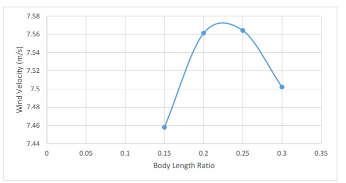
The method used in creating the shroud profile is by solving the ERE curve equations to generate large family of solutions. The system is modeled as axisymmetric system utilizing commercial software package. The effect of the parameters; shroud length, exit diameter, inlet diameter, turbine position with respect to the shroud throat, and wind velocity are studied. An optimum case for each shroud length, exit diameter and location of the shroud with respect to the wind turbine throat axis are achieved.

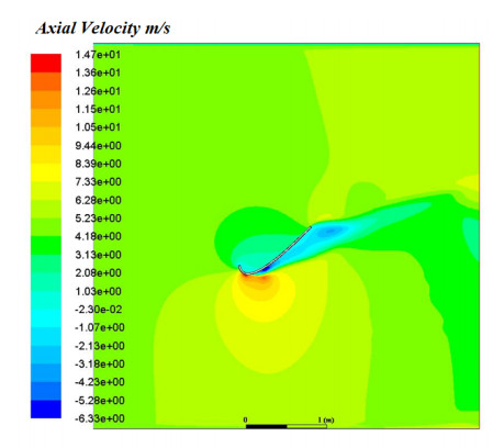
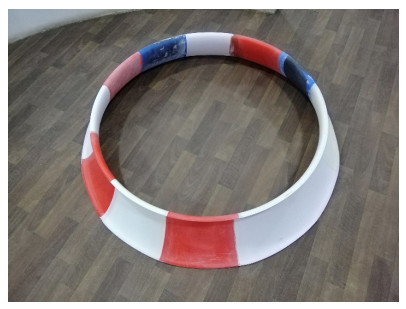
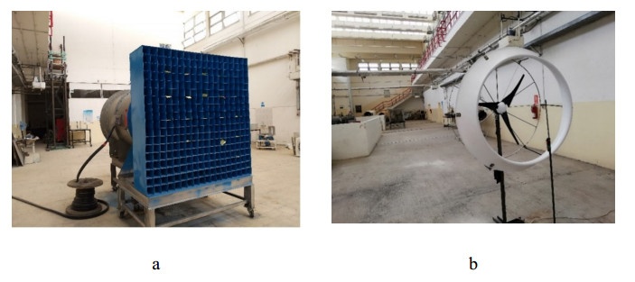
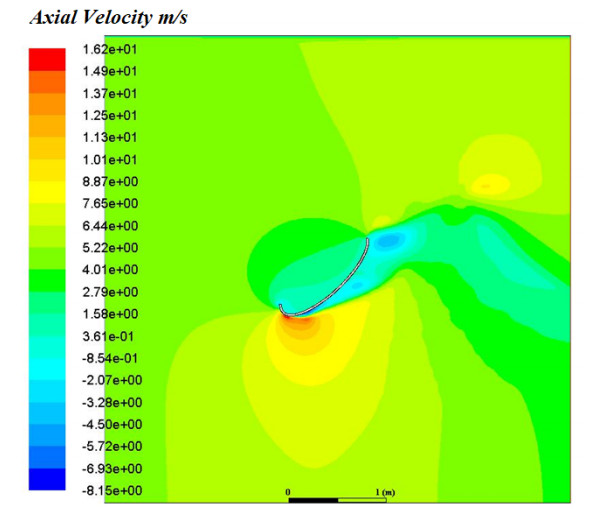
The simulation results show an increase in the average wind velocity by 1.63 times of the inlet velocity. This leads to a great improvement in the wind turbine output power by 4.3 times of bare turbine. One of the achieved optimum solutions for the shroud curves has been prototyped for experimental validation. The prototype has been manufactured using 3D printing technology which provides high accuracy in building the exact shape of shroud design curve. The results show very good agreement with the experimental results.
- wind energy,
- wind lens,
- elliptic shroud,
- low wind speed regions
Citation: Salih Nawaf Akour, Mahmoud Azmi Abo Mhaisen. Parametric design analysis of elliptical shroud profile[J]. AIMS Energy, 2021, 9(6): 1147-1169. doi: 10.3934/energy.2021053

Related Papers:

Abstract

Parametric design analysis for Eccentric Rotated Ellipsoid (ERE) shroud profile is conducted whereas the design model is validated experimentally. A relation between shroud inlet, length and exit diameter is established, different ratios related to the wind turbine diameter are introduced, and solution for different ERE family curves that passes on the inlet, throat, and exit points is studied. The performance of the ERE shroud is studied under different wind velocities ranging from 5–10 m/s.

The method used in creating the shroud profile is by solving the ERE curve equations to generate large family of solutions. The system is modeled as axisymmetric system utilizing commercial software package. The effect of the parameters; shroud length, exit diameter, inlet diameter, turbine position with respect to the shroud throat, and wind velocity are studied. An optimum case for each shroud length, exit diameter and location of the shroud with respect to the wind turbine throat axis are achieved.

The simulation results show an increase in the average wind velocity by 1.63 times of the inlet velocity. This leads to a great improvement in the wind turbine output power by 4.3 times of bare turbine. One of the achieved optimum solutions for the shroud curves has been prototyped for experimental validation. The prototype has been manufactured using 3D printing technology which provides high accuracy in building the exact shape of shroud design curve. The results show very good agreement with the experimental results.

References

[1]	Vries O (1979) Fluid dynamic aspects of wind energy conversion. North Atlantic Treaty Organization Advisory Group for Aerospace Research and Development, Neuilly-sur-Seine France.
[2]	Bontempo R, Manna M (2016) Effects of the duct thrust on the performance of ducted wind turbines. Energy 99: 274-287. doi: 10.1016/j.energy.2016.01.025
[3]	Bontempo R, Manna M (2020) On the potential of the ideal diffuser augmented wind turbine: an investigation by means of a momentum theory approach and of a free-wake ring-vortex actuator disk model. Energy Convers Manage 213: 112794. doi: 10.1016/j.enconman.2020.112794
[4]	Avallone F, Ragni D, Casalino D (2020) On the effect of the tip-clearance ratio on the aeroacoustics of a diffuser-augmented wind turbine. Renewable Energy 152: 1317-1327. doi: 10.1016/j.renene.2020.01.064
[5]	Dighe VV, de Oliveira G, Avallone F, et al. (2019) Characterization of aerodynamic performance of ducted wind turbines: A numerical study. Wind Energy 22: 1655-1666. doi: 10.1002/we.2388
[6]	Venters R, Helenbrook BT, Visser KD (2018) Ducted Wind Turbine Optimization. J Sol Energy Eng 140: 011005. doi: 10.1115/1.4037741
[7]	Bontempo R, Manna M (2020) Diffuser augmented wind turbines: Review and assessment of theoretical models. Appl Energy 280: 115867. doi: 10.1016/j.apenergy.2020.115867
[8]	Ohya Y, Karasudani T, Sakurai A, et al. (2008) Development of a shrouded wind turbine with a flanged diffuser. J Wind Eng Ind Aerodyn 96: 524-539. doi: 10.1016/j.jweia.2008.01.006
[9]	Ohya Y, Karasudani T (2010) A shrouded wind turbine generating high output power with wind-lens technology. Energies 3: 634-649. doi: 10.3390/en3040634
[10]	Srikanth SK (2016) Numerical analysis of wind lens. Int J Innov Res Sci Eng Technol, 5.
[11]	Takahashi S, Hata Y, Ohya Y, et al. (2012) Behavior of the blade tip vortices of a wind turbine equipped with a brimmed-diffuser shroud. Energies 5: 5229-5242. doi: 10.3390/en5125229
[12]	Kosasih B, Tondelli A (2012) Experimental study of shrouded micro-wind turbine. Procedia Eng 49: 92-98. doi: 10.1016/j.proeng.2012.10.116
[13]	Toshimitsu K, Kikugawa H, Sato K, et al. (2012) Experimental investigation of performance of the wind turbine with the flanged-diffuser shroud in sinusoidally oscillating and fluctuating velocity flows. Open J Fluid Dyn 2: 215-221. doi: 10.4236/ojfd.2012.24A024
[14]	Govindharajan R, Parammasivam KM, Vivel V, et al. (2013) Numerical investigation and design optimization of brimmed diffuser-Wind lens around a wind turbine. Eighth Asia-Pacific Conference on Wind Engineering, 1204-1210.
[15]	Jafari SAH, Kosasih B (2014) Flow analysis of shrouded small wind turbine with a simple frustum diffuser with computational fluid dynamics simulations. J Wind Eng Ind Aerodyn 125: 102-110. doi: 10.1016/j.jweia.2013.12.001
[16]	Kosasih BY, Jafari SA (2014) High-Efficiency shrouded micro wind turbine for urban-built environment. Appl Mech Mater 493: 294-299. doi: 10.4028/www.scientific.net/AMM.493.294
[17]	Maia LAB Experimental and numerical study of a diffuser augmented wind turbine-DAWT. Master thesis, 2014. Available from: https://bibliotecadigital.ipb.pt/handle/10198/11600.
[18]	Sangoor AJ (2015) Experimental and computational study of the performance of a new shroud design for an axial wind turbine. Available from: https://etd.ohiolink.edu/apexprod/rws_olink/r/1501/10?clear=10&p10_accession_num=ysu1433503872.
[19]	Liu J, Song M, Chen K, et al. (2016) An optimization methodology for wind lens profile using Computational Fluid Dynamics simulation. Energy 109: 602-611. doi: 10.1016/j.energy.2016.04.131
[20]	Jenkins PE, Younis A, Jenkins PE, et al. (2016) Flow simulation to determine the effects of shrouds on the performance of wind turbines. J Power Energy Eng 4: 79-93. doi: 10.4236/jpee.2016.48008
[21]	Oka N, Furukawa M, Kawamitsu K, et al. (2016) Optimum aerodynamic design for wind-lens turbine. J Fluid Sci Technol 11: JFST0011-JFST0011. doi: 10.1299/jfst.2016jfst0011
[22]	El-Zahaby AM, Kabeel AE, Elsayed SS, et al. (2017) CFD analysis of flow fields for shrouded wind turbine's diffuser model with different flange angles. Alexandria Eng J 56: 171-179. doi: 10.1016/j.aej.2016.08.036
[23]	Ohya Y, Karasudani T, Nagai T, et al. (2017) Wind lens technology and its application to wind and water turbine and beyond. Renewable Energy Environ Sustainability 2: 2. doi: 10.1051/rees/2016022
[24]	Chapra S, Canale R (2006) Numerical Methods for Engineers, McGraw-Hill. 6 Eds, New York: McGraw-Hill.

Reader Comments

Your name:*

Email:*
© 2021 the Author(s), licensee AIMS Press. This is an open access article distributed under the terms of the Creative Commons Attribution License (http://creativecommons.org/licenses/by/4.0)