This article aims to examine the |S11| parameter of a multiband Coplanar Waveguide (CPW)-fed antenna. The proposed square-shaped antenna-1 (Ant.1) and antenna-2 (Ant. 2) are primarily composed of three ground terminal stubs: Terminal-1 (T1), Terminal-2 (T2), and Terminal-3 (T3), all of which have an inverted L-shaped radiating patch. The proposed antennas' resonance frequencies (fr) can be adjusted by the electrical dimension and length of the stub resonators, the dielectric constant (εr) of substrate materials, and their appropriate thicknesses. It will have an impact on their return loss (|S11|), Impedance Bandwidth (IBW), radiation pattern, and antenna performance in terms of frequency characteristics, as demonstrated in this article. The proposed structure based on Flame-Retardant fiber glass epoxy (FR4) substrate covered a wideband frequency range from 1.5 to 3.2 GHz, (IBW = 1.7 GHz) and from 3.4 to 3.65 GHz (IBW = 0.25 GHz). The total IBW is 1.95 GHz, at S11 ≤ −10 dB with three resonance frequencies of values fr1 = 1.75, fr2 = 2.65, and fr3 = 3.50 GHz) for triple-band applications. The results are compared with the research work reported earlier. The proposed Ant.1 ensured, dual and triple band applications whereas the proposed Ant. 2 ensured dual, triple and quad bands applications with reasonable antennas' sizes similar to the earlier reported works. Furthermore, the impacts of various substrate materials as well as different lengths of multi-stub resonators on the operating bands and resonance frequency are thoroughly explored and analyzed for these antennas.
Citation: Sandeep Kumar Singh, Tripurari Sharan, Arvind Kumar Singh. Investigating the S-parameter (|S11|) of CPW-fed antenna using four different dielectric substrate materials for RF multiband applications[J]. AIMS Electronics and Electrical Engineering, 2022, 6(3): 198-222. doi: 10.3934/electreng.2022013
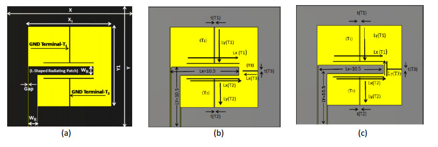
This article aims to examine the |S11| parameter of a multiband Coplanar Waveguide (CPW)-fed antenna. The proposed square-shaped antenna-1 (Ant.1) and antenna-2 (Ant. 2) are primarily composed of three ground terminal stubs: Terminal-1 (T1), Terminal-2 (T2), and Terminal-3 (T3), all of which have an inverted L-shaped radiating patch. The proposed antennas' resonance frequencies (fr) can be adjusted by the electrical dimension and length of the stub resonators, the dielectric constant (εr) of substrate materials, and their appropriate thicknesses. It will have an impact on their return loss (|S11|), Impedance Bandwidth (IBW), radiation pattern, and antenna performance in terms of frequency characteristics, as demonstrated in this article. The proposed structure based on Flame-Retardant fiber glass epoxy (FR4) substrate covered a wideband frequency range from 1.5 to 3.2 GHz, (IBW = 1.7 GHz) and from 3.4 to 3.65 GHz (IBW = 0.25 GHz). The total IBW is 1.95 GHz, at S11 ≤ −10 dB with three resonance frequencies of values fr1 = 1.75, fr2 = 2.65, and fr3 = 3.50 GHz) for triple-band applications. The results are compared with the research work reported earlier. The proposed Ant.1 ensured, dual and triple band applications whereas the proposed Ant. 2 ensured dual, triple and quad bands applications with reasonable antennas' sizes similar to the earlier reported works. Furthermore, the impacts of various substrate materials as well as different lengths of multi-stub resonators on the operating bands and resonance frequency are thoroughly explored and analyzed for these antennas.

| [1] |
Blostein SD, Leib H (2003) Multiple antenna systems: their role and impact in future wireless access. IEEE Commun Mag 41: 94–101. https://doi.org/10.1109/MCOM.2003.1215645 doi: 10.1109/MCOM.2003.1215645

|
| [2] |
Li X, Shi XW, Hu W, et al. (2013) Compact Triband ACS-Fed Monopole Antenna Employing Open-Ended Slots for Wireless Communication. IEEE Antenn Wirel Pr 12: 388–391. https://doi.org/10.1109/LAWP.2013.2252414 doi: 10.1109/LAWP.2013.2252414
|
| [3] |
Chen H, Yang X, Yin YZ, et al. (2013) Triband Planar Monopole Antenna with Compact Radiator for WLAN/WiMAX Applications. IEEE Antenn Wirel Pr 2: 1440–1443. https://doi.org/10.1109/LAWP.2013.2287312 doi: 10.1109/LAWP.2013.2287312
|
| [4] |
Peng CM, Chen IF, Yeh JW (2013) Printed Broadband Asymmetric Dual-Loop Antenna for WLAN/ Wi-MAX Applications. IEEE Antenn Wirel Pr 12: 898–901. https://doi.org/10.1109/LAWP.2013.2273231 doi: 10.1109/LAWP.2013.2273231
|
| [5] |
Dang L, Lei ZY, Xie YJ, et al. (2010) A Compact Microstrip Slot Triple-Band Antenna for WLAN/WiMAX Applications. IEEE Antenn Wirel Pr 9: 1178–1181. https://doi.org/10.1109/LAWP.2010.2098433 doi: 10.1109/LAWP.2010.2098433
|
| [6] |
Wu CM, Chiu CN, Hsu CK (2006) A new non-uniform meandered and fork-type grounded antenna for triple-band WLAN applications. IEEE Antenn Wirel Pr 5: 346–348. https://doi.org/10.1109/LAWP.2006.880692 doi: 10.1109/LAWP.2006.880692
|
| [7] |
Peng L, Ruan C, Wu X (2010) Design and Operation of Dual/Triple-Band Asymmetric M-Shaped Microstrip Patch Antennas. IEEE Antenn Wirel Pr 9: 1069–1072. https://doi.org/10.1109/LAWP.2010.2091671 doi: 10.1109/LAWP.2010.2091671
|
| [8] |
Reddy BR, Vakula D (2015) Compact Zigzag-Shaped-Slit Microstrip Antenna with Circular Defected Ground Structure for Wireless Applications. IEEE Antenn Wirel Pr 14: 678–681. https://doi.org/10.1109/LAWP.2014.2376984 doi: 10.1109/LAWP.2014.2376984
|
| [9] |
Dabas T, Kanaujia BK, Gangwar D, et al. (2018) Design of multiband multi-polarised single feed patch antenna. IET Microw Antenna P 12: 2372–2378. https://doi.org/10.1049/iet-map.2018.5401 doi: 10.1049/iet-map.2018.5401
|
| [10] |
Manouare AZ, Ibnyaich S, Seetharamdoo D, et al. (2019) Design, Fabrication and Measurement of a Novel Compact Triband CPW-Fed Planar Monopole Antenna Using Multi-type Slots for Wireless Communication Applications. J Circuit Syst Comp 29: 1–23. https://doi.org/10.1142/S0218126620500322 doi: 10.1142/S0218126620500322
|
| [11] |
Singla G, Khanna R, Parkash D (2019) CPW fed rectangular rings-based patch antenna with DGS for WLAN/UNII applications. Int J Microw Wirel T 11: 523–531. https://doi.org/10.1017/S1759078719000023 doi: 10.1017/S1759078719000023
|
| [12] |
Yassini AE, Ibnyaich S, Chabaa S, et al. (2020) Miniaturized broadband multiband planar antenna with a symmetric quarter circular ground plane for WLAN/WiMAX standards. Microw Opt Techn Let 10: 1–12. https://doi.org/10.1002/mop.32402 doi: 10.1002/mop.32402
|
| [13] |
Bendahmane Z, Ferouani S, Sayah C (2020) High Permittivity Substrate and DGS Technique for Dual-Band Star-Shape Slotted Microstrip Patch Antenna Miniaturization. Progress In Electromagnetics Research C 102: 163–174. https://doi.org/10.2528/PIERC20021501 doi: 10.2528/PIERC20021501
|
| [14] |
Ansal KA, Kumar AS, Baby SM (2021) Comparative analysis of CPW fed antenna with different substrate material with varying thickness. Materials Today: Proceedings 37: 257–264. https://doi.org/10.1016/j.matpr.2020.05.201 doi: 10.1016/j.matpr.2020.05.201
|
| [15] |
Fu Q, Feng Q, Chen H (2021) Design and Optimization of CPW-Fed Broadband Circularly Polarized Antenna for Multiple Communication Systems. Progress In Electromagnetics Research Letters 99: 65–74. https://doi.org/10.2528/PIERL21062205 doi: 10.2528/PIERL21062205
|
| [16] |
Ma R, Feng Q (2021) Design of Broadband Circularly Polarized Square Slot Antenna for UHF RFID Applications. Progress In Electromagnetics Research C 111: 97–108. https://doi.org/10.2528/PIERC21021403 doi: 10.2528/PIERC21021403
|
| [17] |
Singh SK, Sharan T, Singh AK (2020) A comparative performance analysis of various shapes and substrate materials loaded coplanar waveguide-fed antennas. Materials Today: Proceedings 34: 643–648. https://doi.org/10.1016/j.matpr.2020.03.133 doi: 10.1016/j.matpr.2020.03.133
|
| [18] |
Singh SK, Sharan T, Singh AK (2021) Miniaturization of CPW-Fed Patch Antenna by Using Dielectric Materials for 2.4 GHz (WLAN/ISM) Applications. Macromolecular Symposia 397: 1–10. https://doi.org/10.1002/masy.202100008 doi: 10.1002/masy.202100008
|
| [19] |
Dejen A, Jayasinghe J, Ridwan M, et al. (2022) Genetically engineered tri-band microstrip antenna with improved directivity for mm-wave wireless application. AIMS Electronics and Electrical Engineering 6: 1–15. https://doi.org/10.3934/electreng.2022001 doi: 10.3934/electreng.2022001
|
| [20] |
Ullah MH, Islam MT, Mandeep JS (2013) A parametric study of high dielectric material substrate for small antenna design. Int J Appl Electrom 41: 193–198. https://doi.org/10.3233/JAE-2012-1603 doi: 10.3233/JAE-2012-1603
|
| [21] |
Raveendran A, Sebastian MT, Raman S (2019) Applications of Microwave Materials: A Review. J Electron Mater 48: 2601–2634. https://doi.org/10.1007/s11664-019-07049-1 doi: 10.1007/s11664-019-07049-1
|
| [22] |
Fechine PBA, Tavora A, Kretly LC, et al. (2006) Microstrip antenna on a high dielectric constant substrate: BaTiO3 (BTO)-CaCu3Ti4O12(CCTO) composite screen-printed thick films. J Electron Mater 35: 1848–1856. https://doi.org/10.1007/s11664-006-0167-0 doi: 10.1007/s11664-006-0167-0
|
| [23] |
Toma RN, Shohagh IA, Hasan MN (2019) Analysis of the effect of Changing Height of Substrate of Square Shaped Microstrip Patch Antenna on the Performance for 5G Application. Int J Microw Wirel T 9: 33–45. https://doi.org/10.5815/ijwmt.2019.03.04 doi: 10.5815/ijwmt.2019.03.04
|
| [24] |
Kumar A, Jhanwar D, Sharma MM (2017) A compact printed multistubs loaded resonator rectangular monopole antenna design for multiband wireless systems. Int J RF Microw C E 27: 1–10. https://doi.org/10.1002/mmce.21147 doi: 10.1002/mmce.21147
|
| [25] |
Sharma MM, Deegwal JK, Govil MC, et al. (2015) Compact printed ultra-wideband antenna with two notched stop bands for WiMAX and WLAN. Int J Appl Electrom 47: 523–532. https://doi.org/10.3233/JAE-140007 doi: 10.3233/JAE-140007
|


Figures(19) / Tables(9)

Sandeep Kumar Singh, Tripurari Sharan, Arvind Kumar Singh. Investigating the S-parameter (|S11|) of CPW-fed antenna using four different dielectric substrate materials for RF multiband applications[J]. AIMS Electronics and Electrical Engineering, 2022, 6(3): 198-222. doi: 10.3934/electreng.2022013


 DownLoad: