Estimating complexity of spike-wave discharges with largest Lyapunov exponent in computational models and experimental data

T. M. Medvedeva; A. K. Lüttjohann; M. V. Sysoeva; G. van Luijtelaar; I. V. Sysoev; T. M. Medvedeva; A. K. Lüttjohann; M. V. Sysoeva; G. van Luijtelaar; I. V. Sysoev

doi:10.3934/biophy.2020006

AIMS Biophysics

2020, Volume 7, Issue 2: 65-75. doi: 10.3934/biophy.2020006

Previous Article Next Article

Research article Special Issues

Estimating complexity of spike-wave discharges with largest Lyapunov exponent in computational models and experimental data

1.
Saratov Branch of Kotel'nokov Institute of Radioengineering and Electronics of Russian Academy of Sciences, 38 Zelyonaya str., Saratov, Russia
2.
Institute of Higher Nervous Activity and Neurophysiology of Russian Academy of Sciences, 5A Butlerova str., Moscow, Russia
3.
Saratov State University, 83 Astrakhanskaya str., Saratov, Russia
4.
Institute of Physiology I, Westfalische Wilhelms Universität, 27a Robert-Koch-Strabe, Münster, Germany
5.
Yuri Gagarin State Technical University of Saratov, 77 Politekhnicheskaya str., Saratov, Russia
6.
Donders Centre for Cognition, Radboud University, Nijmegen, P.O.Box 9104 6500 HE, Nijmegen, the Netherlands

Received: 14 February 2020 Accepted: 29 March 2020 Published: 07 April 2020

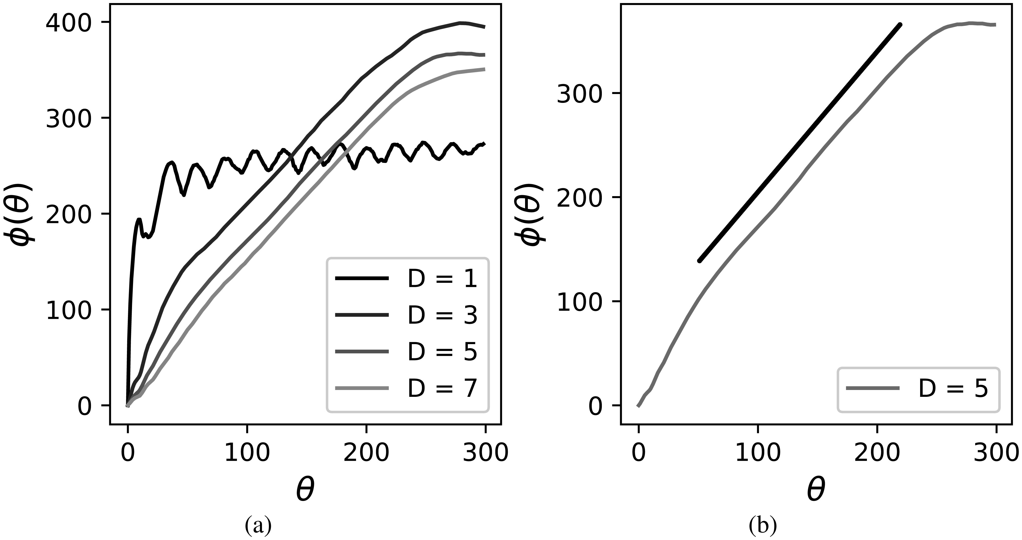
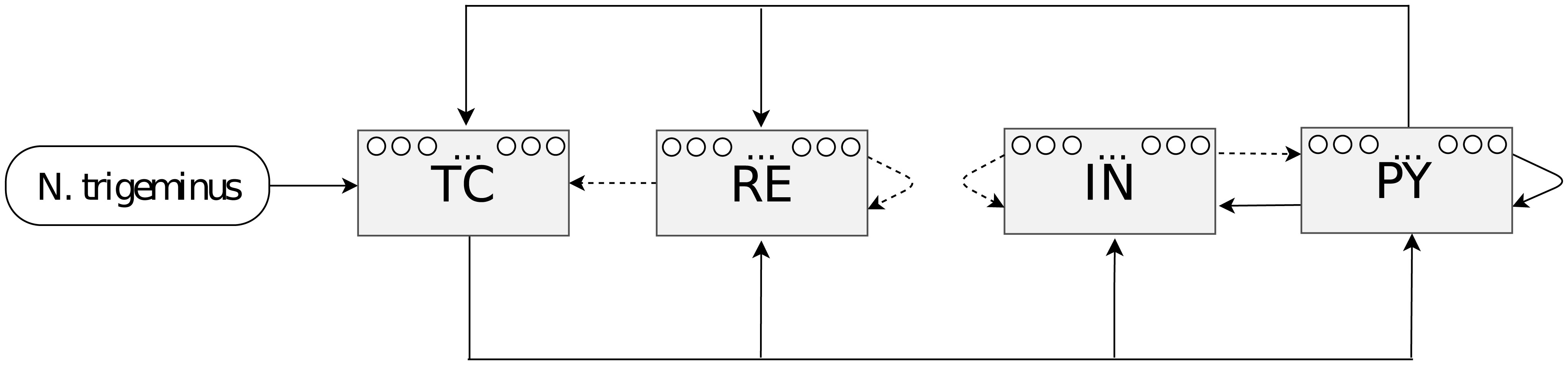
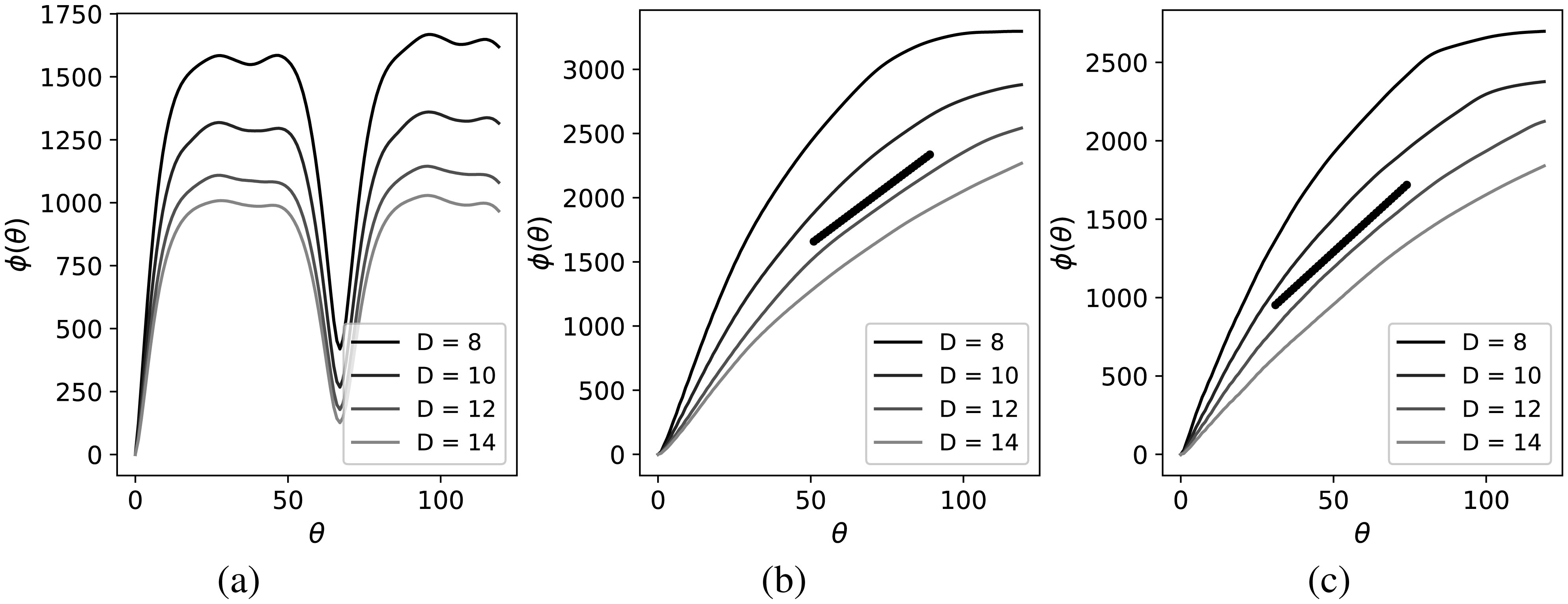
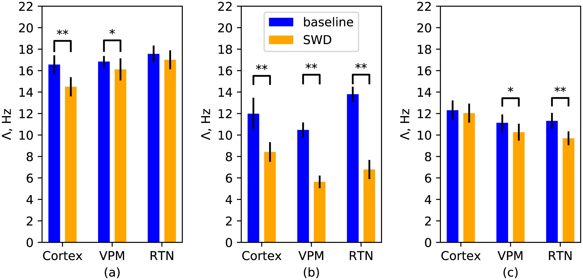
Here we consider the possibility to characterize the signal complexity of electroencephalograms using calculation of largest Lyapunov exponent explicitly from time series. This would help in detection of seizures, understanding and modeling epileptic activity. Baseline activity and spike-wave discharges (SWDs) were considered as regimes. Three channels relevant for absence epilepsy were studied: the parietal cortex, the ventroposterial medial nucleus of thalamus, and the reticular thalamic nucleus. Experimental data and two types of models were investigated. The result show that SWDs often treated as more or less regular oscillations are characterized by large positive Lyapunov exponent, not very different from the value obtained for baseline activity. The mesoscale network model of epilepsy is mostly able to reproduce this phenomenon, including absolute values. The more simple neuron mass model exhibits Lyapunov exponent during SWDs twice smaller than in baseline.
- absence epilepsy,
- Lyapunov exponent,
- time series analysis,
- EEG,
- spike-wave discharges,
- genetic absence epilepsy model,
- computational models
Citation: T. M. Medvedeva, A. K. Lüttjohann, M. V. Sysoeva, G. van Luijtelaar, I. V. Sysoev. Estimating complexity of spike-wave discharges with largest Lyapunov exponent in computational models and experimental data[J]. AIMS Biophysics, 2020, 7(2): 65-75. doi: 10.3934/biophy.2020006

Related Papers:

Abstract

Here we consider the possibility to characterize the signal complexity of electroencephalograms using calculation of largest Lyapunov exponent explicitly from time series. This would help in detection of seizures, understanding and modeling epileptic activity. Baseline activity and spike-wave discharges (SWDs) were considered as regimes. Three channels relevant for absence epilepsy were studied: the parietal cortex, the ventroposterial medial nucleus of thalamus, and the reticular thalamic nucleus. Experimental data and two types of models were investigated. The result show that SWDs often treated as more or less regular oscillations are characterized by large positive Lyapunov exponent, not very different from the value obtained for baseline activity. The mesoscale network model of epilepsy is mostly able to reproduce this phenomenon, including absolute values. The more simple neuron mass model exhibits Lyapunov exponent during SWDs twice smaller than in baseline.

Acknowledgments

This study was funded by Russian Science Foundation, grant number 19-72-10030.

Conflict of interest

Authors declare no conflict of interests.

References

[1]	Röschke J, Başar E (1988) The EEG is not a simple noise: strange attractors in intracranial structures. Dynamics of Sensory and Cognitive Processing by the Brain Berlin: Springer, 203-216. doi: 10.1007/978-3-642-71531-0_13
[2]	Röschke J, Mann K, Fell J (1994) Nonlinear EEG dynamics during sleep in depression and schizophrenia. Int J Neurosci 75: 271-284. doi: 10.3109/00207459408986309
[3]	Coenen AML, Van Luijtelaar E (2003) Genetic animal models for absence epilepsy: A review of the WAG/Rij strain of rats. Behav Genet 33: 635-655. doi: 10.1023/A:1026179013847
[4]	Lüttjohann A, van Luijtelaar G (2015) Dynamics of networks during absence seizure's on-and offset in rodents and man. Front Physiol 6: 16.
[5]	Meeren H, van Luijtelaar G, da Silva FL, et al. (2005) Evolving concepts on the pathophysiology of absence seizures: the cortical focus theory. Arch Neurol 62: 371-376. doi: 10.1001/archneur.62.3.371
[6]	Bosnyakova D, Gabova A, Kuznetsova G, et al. (2006) Time-frequency analysis of spike-wave discharges using a modified wavelet transform. J Neurosci Meth 154: 80-88. doi: 10.1016/j.jneumeth.2005.12.006
[7]	Mukhin RR (2018) Legacy of Alexander Mikhailovich Lyapunov and nonlinear dynamics. Izvestiya VUZ. Appl Nonlin Dynam 26: 95-120. doi: 10.18500/0869-6632-2018-26-4-95-120
[8]	Gonchenko AS, Gonchenko SV, Kazakov AO, et al. (2017) Mathematical theory of dynamical chaos and its applications: Review, part 1. Pseudohyperbolic attractors. Izvestiya VUZ. Appl Nonlin Dynam 25: 4-36.
[9]	Gonchenko SV, Gonchenko AS, Kazakov AO, et al. (2019) Mathematical theory of dynamical chaos and its applications: Review, part 2. Spiral chaos of three-dimensional flows. Izvestiya VUZ. Appl Nonlin Dynam 27: 7-52. doi: 10.18500/0869-6632-2019-27-5-7-52
[10]	Kim DJ, Jeong J, Chae JH, et al. (2000) An estimation of the first positive Lyapunov exponent of the EEG in patients with schizophrenia. Psychiat Res: Neuroim 98: 177-189. doi: 10.1016/S0925-4927(00)00052-4
[11]	Aftanas LI, Lotova NV, Koshkarov VI, et al. (1997) Non-linear analysis of emotion EEG: calculation of Kolmogorov entropy and the principal Lyapunov exponent. Neurosci Lett 226: 13-16. doi: 10.1016/S0304-3940(97)00232-2
[12]	Röschke J, Fell J, Beckmann P (1993) The calculation of the first positive Lyapunov exponent in sleep EEG data. Electroencephalography Clin Neurophysiol 86: 348-352. doi: 10.1016/0013-4694(93)90048-Z
[13]	van Luijtelaar G, Lüttjohann A, Makarov VV, et al. (2016) Methods of automated absence seizure detection, interference by stimulation, and possibilities for prediction in genetic absence models. J Neurosci Meth 260: 144-158. doi: 10.1016/j.jneumeth.2015.07.010
[14]	Granger CWJ (1969) Investigating causal relations by econometric models and cross-spectral methods. Economet Soc 37: 424-438. doi: 10.2307/1912791
[15]	Hesse W, Möller E, Arnold M, et al. (2003) The use of time-variant EEG Granger causality for inspecting directed interdependencies of neural assemblies. J Neurosci Meth 124: 27-44. doi: 10.1016/S0165-0270(02)00366-7
[16]	Sysoeva MV, Sitnikova E, Sysoev IV, et al. (2014) Application of adaptive nonlinear Granger causality: Disclosing network changes before and after absence seizure onset in a genetic rat model. J Neurosci Meth 226: 33-41. doi: 10.1016/j.jneumeth.2014.01.028
[17]	Schreiber T (2000) Measuring information transfer. Phys Rev Lett 85: 461-464. doi: 10.1103/PhysRevLett.85.461
[18]	Baccalá LA, Sameshima K (2001) Partial directed coherence: a new concept in neural structure determination. Biol Cybern 84: 463-474. doi: 10.1007/PL00007990
[19]	Wolf A, Swift JB, Swinney HL, et al. (1985) Determining Lyapunov exponents from a time series. Physica D 16: 285-317. doi: 10.1016/0167-2789(85)90011-9
[20]	Eckmann JP, Kamphorst SO, Ruelle D, et al. (1986) Liapunov exponents from time series. Phys Rev A 34: 4971-4799. doi: 10.1103/PhysRevA.34.4971
[21]	Meeren HKM, Pijn JPM, van Luijtelaar ELJM, et al. (2002) Cortical focus drives widespread corticothalamic networks during spontaneous absence seizures in rats. J Neurosci 22: 1480-1495. doi: 10.1523/JNEUROSCI.22-04-01480.2002
[22]	Sysoeva MV, Lüttjohann A, van Luijtelaar G, et al. (2016) Dynamics of directional coupling underlying spike-wave discharges. Neuroscience 314: 75-89. doi: 10.1016/j.neuroscience.2015.11.044
[23]	Rosenstein MT, Collins JJ, De Luca CJ (1993) A practical method for calculating largest Lyapunov exponents from small data sets. Physica D 65: 117-134. doi: 10.1016/0167-2789(93)90009-P
[24]	Packard NH, Crutchfield JP, Farmer JD, et al. (1980) Geometry from a Time Series. Phys Rev Lett 45: 712-715. doi: 10.1103/PhysRevLett.45.712
[25]	Kennel MB, Buhl M (2003) Estimating good discrete partitions from observed data: Symbolic false nearest neighbors. Phys Rev Lett 91: 084102. doi: 10.1103/PhysRevLett.91.084102
[26]	Lüttjohann A, van Luijtelaar G (2012) The dynamics of cortico-thalamo-cortical interactions at the transition from pre-ictal to ictal LFPs in absence epilepsy. Neurobiol Dis 47: 49-60. doi: 10.1016/j.nbd.2012.03.023
[27]	Paxinos G, Watson C (2006) The Rat Brain in Stereotaxic Coordinates San Diego: Academic Press.
[28]	Taylor PN, Wang Y, Goodfellow M, et al. (2014) A computational study of stimulus driven epileptic seizure abatement. Plos One 9: e114316. doi: 10.1371/journal.pone.0114316
[29]	Suffczynski P, Kalitzin S, Da Silva FHL (2004) Dynamics of non-convulsive epileptic phenomena modeled by a bistable neuronal network. Neuroscience 126: 467-484. doi: 10.1016/j.neuroscience.2004.03.014
[30]	Amari S (1977) Dynamics of pattern formation in lateral-inhibition type neural fields. Biol Cybern 27: 77-87. doi: 10.1007/BF00337259
[31]	Medvedeva TM, Sysoeva MV, Sysoev IV (2018) Coupling analysis between thalamus and cortex in mesoscale model of spike-wave discharges from time series of summarized activity of model neurons. 2nd School on Dynamics of Complex Networks and their Application in Intellectual Robotics Russia: Saratov.
[32]	Medvedeva TM, Sysoeva MV, van Luijtelaar G, et al. (2018) Modeling spike-wave discharges by a complex network of neuronal oscillators. Neural Networks 98: 271-282. doi: 10.1016/j.neunet.2017.12.002
[33]	FitzHugh R (1961) Impulses and physiological states in theoretical models of nerve membrane. Biophys J 1: 445-466. doi: 10.1016/S0006-3495(61)86902-6
[34]	Nagumo J, Arimoto S, Yoshizawa S (1962) An active pulse transmission line simulating nerve axon. P IRE 50: 2061-2070. doi: 10.1109/JRPROC.1962.288235
[35]	Sysoeva MV, Kuznetsova GD, Sysoev IV (2016) The modeling of rat EEG signals in absence epilepsy in the analysis of brain connectivity. Biophysics 61: 661-669. doi: 10.1134/S0006350916040230
[36]	Sitnikova E, Koronovskii AA, Hramov AE (2011) Analysis of epileptic activity of brain in case of absence epilepsy: applied aspects of nonlinear dynamics. Izvestiya VUZ. Appl Nonlinear Dynam 19: 173-182.
[37]	Smyk MK, Sysoev IV, Sysoeva MV, et al. (2019) Can absence seizures be predicted by vigilance states?: Advanced analysis of sleep–wake states and spike–wave discharges' occurrence in rats. Epilepsy Behav 96: 200-209. doi: 10.1016/j.yebeh.2019.04.012

Reader Comments

Your name:*

Email:*
© 2020 the Author(s), licensee AIMS Press. This is an open access article distributed under the terms of the Creative Commons Attribution License (http://creativecommons.org/licenses/by/4.0)