Cultured meat: A survey of awareness among Greek consumers

Andriana E. Lazou; Panagiota-Kyriaki Revelou; Spiridoula Kougioumtzoglou; Irini F. Strati; Anastasia Kanellou; Anthimia Batrinou; Andriana E. Lazou; Panagiota-Kyriaki Revelou; Spiridoula Kougioumtzoglou; Irini F. Strati; Anastasia Kanellou; Anthimia Batrinou

doi:10.3934/agrfood.2024021

AIMS Agriculture and Food

2024, Volume 9, Issue 1: 356-373. doi: 10.3934/agrfood.2024021

Previous Article Next Article

Research article Special Issues

Cultured meat: A survey of awareness among Greek consumers

1.
Laboratory of Chemistry, Analysis & Design of Food Processes, Department of Food Science and Technology, School of Food Sciences, University of West Attica, 12243 Athens, Greece
2.
Laboratory of Chemistry, Department of Food Science and Human Nutrition, Agricultural University of Athens EU-CONEXUS European University, 11855 Athens, Greece
3.
Laboratory of Quality Control & Safety of Foods and Drinks, Department of Food Science and Technology, School of Food Sciences, University of West Attica, 12243 Athens, Greece
^# Equally contributing authors

Received: 01 December 2023 Revised: 02 February 2024 Accepted: 26 February 2024 Published: 13 March 2024

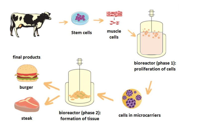
As the technology of cultured meat continues to evolve and reach the market, it is important to understand the dynamics of consumer attitudes and preferences in order to provide insights into the potential adoption of cultured meat in Europe. Our aim was to explore the attitudes of Greek consumers, via an online survey addressed to 1230 consumers. The results revealed that only 39.35% of participants in this survey were aware of the term "cultured meat", but 55.69% would be willing to try it with the group of young (18–25 years old) being more willing to try compared to > 25 years old and also male and graduates. Among the perceived benefits, the first rated benefit was the contribution to animal welfare, followed by the lower environmental impact of cultured meat. The highest concerns about the potential negative consequences of cultured meat were about the unknown long-term adverse health effects and about a negative impact on the local livestock producers. Most of the respondents (80.73%) agreed that cultured meat is an artificial product. In conclusion, our results revealed a level of skepticism and reservations regarding cultured meat among Greek consumers and addressing public concerns might be especially important to increase public acceptance of cultured meat.
- animal welfare,
- attitudes,
- cultured meat,
- environmental impact,
- preferences,
- survey
Citation: Andriana E. Lazou, Panagiota-Kyriaki Revelou, Spiridoula Kougioumtzoglou, Irini F. Strati, Anastasia Kanellou, Anthimia Batrinou. Cultured meat: A survey of awareness among Greek consumers[J]. AIMS Agriculture and Food, 2024, 9(1): 356-373. doi: 10.3934/agrfood.2024021

Related Papers:

Abstract

As the technology of cultured meat continues to evolve and reach the market, it is important to understand the dynamics of consumer attitudes and preferences in order to provide insights into the potential adoption of cultured meat in Europe. Our aim was to explore the attitudes of Greek consumers, via an online survey addressed to 1230 consumers. The results revealed that only 39.35% of participants in this survey were aware of the term "cultured meat", but 55.69% would be willing to try it with the group of young (18–25 years old) being more willing to try compared to > 25 years old and also male and graduates. Among the perceived benefits, the first rated benefit was the contribution to animal welfare, followed by the lower environmental impact of cultured meat. The highest concerns about the potential negative consequences of cultured meat were about the unknown long-term adverse health effects and about a negative impact on the local livestock producers. Most of the respondents (80.73%) agreed that cultured meat is an artificial product. In conclusion, our results revealed a level of skepticism and reservations regarding cultured meat among Greek consumers and addressing public concerns might be especially important to increase public acceptance of cultured meat.

References

[1]	OECD (2021) OECD-FAO Agricultural Outlook 2021-2030. OECD Publishing: Paris.
[2]	Siegrist M, Sütterlin B, Hartmann C (2018) Perceived naturalness and evoked disgust influence acceptance of cultured meat. Meat Sci 139: 213–219.
[3]	Michel F, Siegrist M (2019) How should importance of naturalness be measured? A comparison of different scales. Appetite 140: 298–304.
[4]	McNamara E, Bomkamp C (2022) Cultivated meat as a tool for fighting antimicrobial resistance. Nat Food 3: 791–794.
[5]	Treich N (2021) Cultured meat: Promises and challenges. Environ Resour Econ 79: 33–61.
[6]	Zhang G, Zhao X, Li X, et al. (2020) Challenges and possibilities for bio-manufacturing cultured meat. Trends Food Sci Technol 97: 443–450.
[7]	Stephens N, Sexton AE, Driessen C (2019) Making Sense of making meat: Key moments in the first 20 years of tissue engineering muscle to make food. Front Sustain Food Syst 3: 45. https://doi.org/10.3389/fsufs.2019.00045 doi: 10.3389/fsufs.2019.00045
[8]	Lee DY, Lee SY, Jung JW, et al. (2022) Review of technology and materials for the development of cultured meat. Crit Rev Food Sci Nutr 63: 8591–8615. https://doi.org/10.1080/10408398.2022.2063249 doi: 10.1080/10408398.2022.2063249
[9]	Bryant C, Barnett J (2020) Consumer acceptance of cultured meat: An updated review (2018–2020). Appl Sci 10: 5201.
[10]	Boereboom A, Mongondry P, de Aguiar LK, et al. (2022) Identifying consumer groups and their characteristics based on their willingness to engage with cultured meat: A comparison of four European countries. Foods 11: 197.
[11]	IMARC Group (2023) Cultured Meat Market: Global Industry Trends, Share, Size, Growth, Opportunity and Forecast 2023–2028. Available from: https://www.researchandmarkets.com/reports/5820553/cultured-meat-market-global-industry-trends.
[12]	Wilks M, Phillips CJC, Fielding K, et al. (2019) Testing potential psychological predictors of attitudes towards cultured meat. Appetite 136: 137–145.
[13]	Wilks M, Phillips CJC (2017) Attitudes to in vitro meat: A survey of potential consumers in the United States. PLoS One 12: e0171904.
[14]	Shaw E, Mac Con Iomaire M (2019) A comparative analysis of the attitudes of rural and urban consumers towards cultured meat. Br Food J 121: 1782–1800. https://doi.org/10.1108/BFJ-07-2018-0433 doi: 10.1108/BFJ-07-2018-0433
[15]	Mancini MC, Antonioli F (2019) Exploring consumers' attitude towards cultured meat in Italy. Meat Sci 150: 101–110.
[16]	Gómez-Luciano CA, de Aguiar LK, Vriesekoop F, et al. (2019) Consumers' willingness to purchase three alternatives to meat proteins in the United Kingdom, Spain, Brazil and the Dominican Republic. Food Qual Prefer 78: 103732.
[17]	Zhang M, Li L, Bai J (2020) Consumer acceptance of cultured meat in urban areas of three cities in China. Food Control 118: 107390.
[18]	Tucker CA (2014) The significance of sensory appeal for reduced meat consumption. Appetite 81: 168–179.
[19]	Slade P (2018) If you build it, will they eat it? Consumer preferences for plant-based and cultured meat burgers. Appetite 125: 428–437.
[20]	Hocquette A, Lambert C, Sinquin C, et al. (2015) Educated consumers don't believe artificial meat is the solution to the problems with the meat industry. J Integr Agric 14: 273–284.
[21]	Franceković P, García-Torralba L, Sakoulogeorga E, et al. (2021) How do consumers perceive cultured meat in croatia, greece, and spain? Nutrients 13: 1284. https://doi.org/10.3390/nu13041284 doi: 10.3390/nu13041284
[22]	van der Weele C, Driessen C (2019) How normal meat becomes stranger as cultured meat becomes more normal; ambivalence and ambiguity below the surface of behavior. Front Sustain Food Syst 3: 69. https://doi.org/10.3389/fsufs.2019.00069 doi: 10.3389/fsufs.2019.00069
[23]	Weinrich R, Strack M, Neugebauer F (2020) Consumer acceptance of cultured meat in Germany. Meat Sci 162: 107924.
[24]	Circus VE, Robison R (2019) Exploring perceptions of sustainable proteins and meat attachment. Br Food J 121: 533–545.
[25]	Valente J de PS, Fiedler RA, Sucha Heidemann M, et al. (2019) First glimpse on attitudes of highly educated consumers towards cell-based meat and related issues in Brazil. PLoS One 14: e0221129.
[26]	Bryant C, Barnett J (2018) Consumer acceptance of cultured meat: A systematic review. Meat Sci 143: 8–17.
[27]	Lynch J, Pierrehumbert R (2019) Climate impacts of cultured meat and beef cattle. Front Sustain Food Syst 3.
[28]	Tsvakirai CZ, Nalley LL, Tshehla M (2024) What do we know about consumers' attitudes towards cultured meat? A scoping review. Future Foods 9: 100279. https://doi.org/10.1016/j.fufo.2023.100279 doi: 10.1016/j.fufo.2023.100279
[29]	Mancini MC, Antonioli F (2020) To what extent are consumers' perception and acceptance of alternative meat production systems affected by information? The case of cultured meat. Animals 10: 656.
[30]	Laestadius LI, Caldwell MA (2015) Is the future of meat palatable? Perceptions of in vitro meat as evidenced by online news comments. Public Health Nutr 18: 2457–2467.
[31]	Lupton D, Turner B (2018) Food of the future? consumer responses to the idea of 3d-printed meat and insect-based foods. Food Foodways 26: 269–289.
[32]	Verbeke W, Marcu A, Rutsaert P, et al. (2015) 'Would you eat cultured meat?': Consumers' reactions and attitude formation in Belgium, Portugal and the United Kingdom. Meat Sci 102: 49–58.
[33]	Bryant C, Szejda K, Parekh N, et al. (2019) A survey of consumer perceptions of plant-based and clean meat in the USA, India, and China. Front Sustain Food Syst 3: 11. https://doi.org/10.3389/fsufs.2019.00011 doi: 10.3389/fsufs.2019.00011
[34]	Dupont J, Fiebelkorn F (2020) Attitudes and acceptance of young people toward the consumption of insects and cultured meat in Germany. Food Qual Prefer 85: 103983.
[35]	Egolf A, Hartmann C, Siegrist M (2019) When Evolution Works Against the Future: Disgust's Contributions to the Acceptance of New Food Technologies. Risk Anal 39: 1546–1559.
[36]	Popescu A, Dinu TA, Stoian E, et al. (2022) Livestock decline and animal output growth in the European Union in the period 2012–2021. Sci Pap Ser Manage Econ Eng Agric Rural Dev 22: 503–514.
[37]	Garrison GL, Biermacher JT, Brorsen BW (2022) How much will large-scale production of cell-cultured meat cost? J Agric Food Res 10: 100358. https://doi.org/10.1016/j.jafr.2022.100358 doi: 10.1016/j.jafr.2022.100358
[38]	O'Keefe L, McLachlan C, Gough C, et al. (2016) Consumer responses to a future UK food system. Br Food J 118: 412–428.
[39]	Rolland NCM, Markus CR, Post MJ (2020) The effect of information content on acceptance of cultured meat in a tasting context. PLoS One 15: e0231176.
[40]	Rombach M, Dean D, Vriesekoop F, et al. (2022) Is cultured meat a promising consumer alternative? Exploring key factors determining consumer's willingness to try, buy and pay a premium for cultured meat. Appetite 179: 106307. https://doi.org/10.1016/j.appet.2022.106307 doi: 10.1016/j.appet.2022.106307
[41]	Kantor BN, Kantor J (2021) Public attitudes and willingness to pay for cultured meat: A cross-sectional experimental study. Front Sustain Food Syst 5: 594650. http://dx.doi.org/10.3389/fsufs.2021.594650 doi: 10.3389/fsufs.2021.594650

Reader Comments

Your name:*

Email:*
© 2024 the Author(s), licensee AIMS Press. This is an open access article distributed under the terms of the Creative Commons Attribution License (http://creativecommons.org/licenses/by/4.0)