Bioactive and nutritional compounds in fruits of pepper (<i>Capsicum annuum</i> L.) landraces conserved among indigenous communities from Mexico

Rosalía García-Vásquez; Araceli Minerva Vera-Guzmán; José Cruz Carrillo-Rodríguez; Mónica Lilian Pérez-Ochoa; Elia Nora Aquino-Bolaños; Jimena Esther Alba-Jiménez; José Luis Chávez-Servia; Rosalía García-Vásquez; Araceli Minerva Vera-Guzmán; José Cruz Carrillo-Rodríguez; Mónica Lilian Pérez-Ochoa; Elia Nora Aquino-Bolaños; Jimena Esther Alba-Jiménez; José Luis Chávez-Servia

doi:10.3934/agrfood.2023044

AIMS Agriculture and Food

2023, Volume 8, Issue 3: 832-850. doi: 10.3934/agrfood.2023044

Previous Article Next Article

Research article

Bioactive and nutritional compounds in fruits of pepper (Capsicum annuum L.) landraces conserved among indigenous communities from Mexico

1.
Instituto Tecnológico del Valle de Oaxaca, Oaxaca, México
2.
CIIDIR-Oaxaca, Instituto Politécnico Nacional, Oaxaca, México
3.
Centro de Investigación y Desarrollo en Alimentos, Universidad Veracruzana, Veracruz, México
4.
Centro de Investigación y Desarrollo en Alimentos, CONACyT-Universidad Veracruzana, Veracruz, México

Received: 10 April 2023 Revised: 25 July 2023 Accepted: 17 August 2023 Published: 31 August 2023

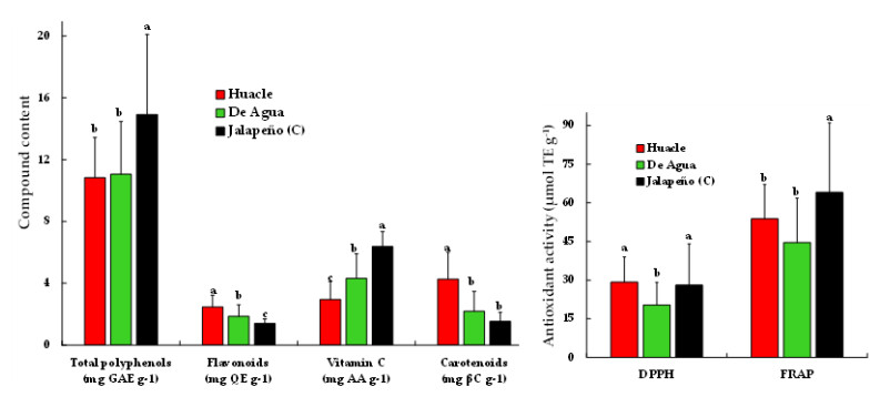
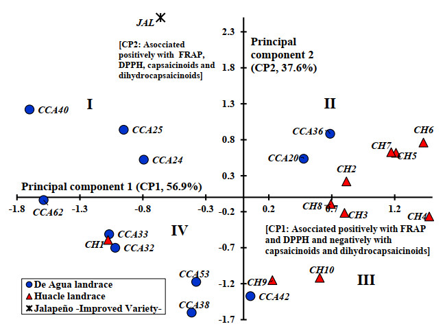
Farmers' varieties or landraces of chili are regularly heterogeneous, selected and preserved by small traditional farmers and highly demanded by regional consumers. The objective of this study was to evaluate the variation in the content of phenolic compounds, vitamin C, carotenoids, capsaicinoids and antioxidant activity in fruits of a population collection of the landraces Huacle and De Agua, which originated in Oaxaca, Mexico, and a commercial variety of Jalapeño (control). The collection was grown in greenhouse conditions under a random block design. At harvest, a sample of ripe fruits was obtained to evaluate the content of phenolic compounds, vitamin C and antioxidant activity by UV–visible spectrophotometry and the concentration of capsaicin and dihydrocapsaicin was measured by high-resolution liquid chromatography. Significant differences were observed between the Huacle and De Agua landraces and between these and Jalapeño. The studied fruits exhibit the following pattern for flavonoid and carotenoid contents: Huacle > De Agua > Jalapeño. The opposite pattern was observed for total polyphenol and vitamin C contents: Jalapeño > De Agua > Huacle. The general pattern for capsaicinoids in fruits was Jalapeño > De Agua > Huacle. Huacle and De Agua populations showed high variability in all compounds evaluated, with positive correlations with antioxidant activity. The capsaicin content in Huacle populations varied ranging from 7.4 to 26.2 mg 100 g^-1 and De Agua ranged from 12.4 to 46.8 mg 100 g^-1.

Keywords:

Citation: Rosalía García-Vásquez, Araceli Minerva Vera-Guzmán, José Cruz Carrillo-Rodríguez, Mónica Lilian Pérez-Ochoa, Elia Nora Aquino-Bolaños, Jimena Esther Alba-Jiménez, José Luis Chávez-Servia. Bioactive and nutritional compounds in fruits of pepper (Capsicum annuum L.) landraces conserved among indigenous communities from Mexico[J]. AIMS Agriculture and Food, 2023, 8(3): 832-850. doi: 10.3934/agrfood.2023044

Related Papers:

[1]	Tao-Li Kang, Hai-Feng Huo, Hong Xiang . Dynamics and optimal control of tuberculosis model with the combined effects of vaccination, treatment and contaminated environments. Mathematical Biosciences and Engineering, 2024, 21(4): 5308-5334. doi: 10.3934/mbe.2024234
[2]	Benjamin H. Singer, Denise E. Kirschner . Influence of backward bifurcation on interpretation of $R_0$ in a model of epidemic tuberculosis with reinfection. Mathematical Biosciences and Engineering, 2004, 1(1): 81-93. doi: 10.3934/mbe.2004.1.81
[3]	Siyu Liu, Yong Li, Yingjie Bi, Qingdao Huang . Mixed vaccination strategy for the control of tuberculosis: A case study in China. Mathematical Biosciences and Engineering, 2017, 14(3): 695-708. doi: 10.3934/mbe.2017039
[4]	Silvia Martorano Raimundo, Hyun Mo Yang, Ezio Venturino . Theoretical assessment of the relative incidences of sensitive andresistant tuberculosis epidemic in presence of drug treatment. Mathematical Biosciences and Engineering, 2014, 11(4): 971-993. doi: 10.3934/mbe.2014.11.971
[5]	Luju Liu, Jianhong Wu, Xiao-Qiang Zhao . The impact of migrant workers on the tuberculosis transmission: General models and a case study for China. Mathematical Biosciences and Engineering, 2012, 9(4): 785-807. doi: 10.3934/mbe.2012.9.785
[6]	Azizeh Jabbari, Carlos Castillo-Chavez, Fereshteh Nazari, Baojun Song, Hossein Kheiri . A two-strain TB model with multiplelatent stages. Mathematical Biosciences and Engineering, 2016, 13(4): 741-785. doi: 10.3934/mbe.2016017
[7]	Zuqin Ding, Yaxiao Li, Xiaomeng Wang, Huling Li, Yongli Cai, Bingxian Wang, Kai Wang, Weiming Wang . The impact of air pollution on the transmission of pulmonary tuberculosis. Mathematical Biosciences and Engineering, 2020, 17(4): 4317-4327. doi: 10.3934/mbe.2020238
[8]	Lih-Ing W. Roeger, Z. Feng, Carlos Castillo-Chávez . Modeling TB and HIV co-infections. Mathematical Biosciences and Engineering, 2009, 6(4): 815-837. doi: 10.3934/mbe.2009.6.815
[9]	Carlos Castillo-Chavez, Baojun Song . Dynamical Models of Tuberculosis and Their Applications. Mathematical Biosciences and Engineering, 2004, 1(2): 361-404. doi: 10.3934/mbe.2004.1.361
[10]	Abba B. Gumel, Baojun Song . Existence of multiple-stable equilibria for a multi-drug-resistant model of mycobacterium tuberculosis. Mathematical Biosciences and Engineering, 2008, 5(3): 437-455. doi: 10.3934/mbe.2008.5.437

Abstract

1. Introduction

Tuberculosis (TB) is an ancient disease with a worldwide distribution and is the leading cause of death from bacterial infections. Mycobacterium TB, is the causative agent of TB. It was discovered and proved to be the causative agent of human TB by the German bacteriologist Koch in 1882, and it can invade all organs of the body, but is most common in causing pulmonary TB. TB is mainly transmitted through the respiratory tract, and the source of infection is through contact with TB patients who have excreted the bacteria ^[1]. In the 19th century, TB became a major epidemic in Europe and elsewhere, spreading to all levels of society and causing one out of every seven deaths, known as the "Great White Plague" ^[2]. Due to the low effectiveness of drugs used to treat TB, the disease is still uncontrollable and remains widespread worldwide. Between 1993 and 1996, the number of TB cases worldwide increased by 13% and TB killed more people than AIDS and malaria combined. In late 1995, the World Health Organization (WHO) established March 24 as World TB Day to further promote global awareness of TB prevention and control ^[3]. Approximately 80% of new TB cases worldwide occur in 22 high-burden countries, with the largest number of global cases accounted to India with 26% and China with 12%, respectively ^[4]. To this day, TB remains the leading cause of disease and death in most high-incidence countries ^[3]. To end the global TB epidemic, WHO proposed in 2014 a post-2015 global end-TB strategy target of a 50% reduction in TB incidence by 2025 (compared to 2015) and a 90% reduction in new cases by 2035.

Mathematical models have become a powerful tool for analyzing epidemiological characteristics ^[5]. Many scholars developed mathematical models reflecting the characteristics of TB based on its transmission mechanism, principles of biology, seasonal characteristics and social influences. In 1962, Waaler developed the first model of TB transmission kinetics ^[6]. In 1967 Brogger further refined Waaler's model. He not only introduced heterogeneity but also changed the method of calculating the incidence rate; however, he did not give the relationship between infection and incidence rates ^[7]. ReVelle developed the first nonlinear differential equation model for TB using Brogger and Waaler's model as a template ^[8]. E. Ziv et al. studied the effect of early treatment on the incidence of TB and found that early treatment reduced the incidence of TB if the treatment rate for active TB was increased from 50% to 60%. Carlos Castillo-Chavez et al. studied the role of mobility and health disparities on the transmission dynamics of TB ^[9]. In addition, medical studies have shown that anti-TB drugs can reduce the length of treatment for TB ^[10]. Meanwhile, many studies have considered the effects of drug-resistant cases ^[11], time lag ^[12] and age structure ^[13]. However, few studies use models of TB with different age groupings. Therefore, based on the collected data and the observed data characteristics (Figure 2), a susceptible-exposed-infectious-recovered (SEIR) model with different age groups is developed, and the feature of heterogeneity is considered in the model to assess the effect of age as a factor on TB transmission.

The main research of this paper is as follows: in section two, the detailed data collected is given and the data in relation is analyzed. A kinetic transmission model is developed, the main parameters in the model are fitted and the value of the basic reproduction number R_v is calculated. In section three, a sensitivity analysis of the basic reproduction number R_v is performed, considering the effect of the proportion of preferential contact within the group on R_v. Finally, a feasibility assessment of the WHO strategic objective of ending TB is presented. Section four contains the discussion section.

2. Materials and methods

2.1. Data analysis

China is one of the high TB burden countries and faces a serious TB epidemic. The burden of TB in China has increased in the last two decades due to the emergence of drug-resistant strains of Mycobacterium TB ^[14], with an average of more than 800,000 new infections per year. The number of new cases from 2004 to 2021 is presented in Figure 1(A), which shows that the number of new infections per year is decreasing each year. A three-dimensional plot of the incidence by age group is given, and it is shows that the incidence of TB in different age groups is significantly different. The incidence rate was lowest in the 0–15 age group and much higher in the 60+ age group compared to other age groups. Overall, the number of TB cases was the highest in the 20–25 and 60–65 age groups, the results of which are shown in Figure 1(B), (C). Statistical data on the morbidity of TB in each age group is shown in Figure 1(D).

Figure 1. Confirmed cases of TB in mainland China in the past two decades. (A) Number of new infections per year. (B) Three-dimensional plot of TB data at different ages. (C) Contour plot of TB data at different ages. (D) Three-dimensional plot of TB morbidity data at different ages.

DownLoad: Full-Size Img PowerPoint

According to the data of the United Nations ^[15], the rate of aging in China is gradually accelerating. The incidence of TB in different age groups was counted, mainly including the mean number of TB incidence, the mean incidence rate and its 95% confidence interval (CI) for each age group in the past fifteen years and the results of statistical analysis, which are shown in Table 1 with the incidence rate in units of 1/100,000. The results show that with the gradual increase of age, the number of TB incidence showed a trend of rising and then decreasing, while the incidence of TB showed a trend of increasing.

Table 1. Number and incidence of TB by age group and their confidence intervals.

Age grouping	Mean number of incidences	95%CI	Mean incidence rate	95%CI
0–5	2692	1645–3738	3.4073	2.0316–4.7830
5–10	3005	1619–4391	3.9197	2.1201–5.7192
10–15	6666	5284–8047	7.8952	7.1978–8.5925
15–20	58,335	51,904–64,766	56.2213	54.8779–57.5647
20–25	97,491	86,176–108,805	83.3704	69.7977–96.9431
25–30	79,469	74,453–84,486	80.3324	71.4972–89.1677
30–35	67,689	56,899–78,479	68.0293	61.3837–74.6749
35–40	69,529	57,746–81,312	59.7398	51.3281–68.1515
40–45	76,188	67,365–85,011	66.8514	57.3751–76.3276
45–50	74,451	71,112–77,790	73.0433	64.3025–81.7842
50–55	80,333	73,185–87,480	95.4184	87.3205–103.5163
55–60	78,587	72,486–84,689	101.3584	88.3025–114.4143
60–65	81,710	78,840–84,580	146.2743	131.4336–161.1151
65–70	71,538	67,286–75,789	170.6339	154.6441–186.6238
70–75	65,196	58,412–71,981	201.5498	172.0765–231.0232
75–80	44,653	41,831–47,474	195.5469	168.0045–223.0892
80–85	21,985	20,706–23,264	175.2472	151.4695–199.0249
85+	8164	7339–8988	163.7941	126.7235–200.8647

| Show Table

DownLoad: CSV

Based on the statistical data from 2004 to 2018, a cluster analysis of the data on the incidence of TB in different age groups is given. The complete classification process for all data is shown in Figure 2 and their complete clustering results are shown in Table 2, where distance refers to a distance between a member of each class and the center of that class, and center, in this case, refers to a concept similar to the mean value within group. The cluster column in the table shows the final clustering results. We obtained the age group 0–15 years is the category with the lowest incidence of TB, the age group 15–60 years is the category with higher incidence and the group over 60 years is the category with the highest incidence.

Figure 2. Clustered analysis of incidence data for different age groups.

DownLoad: Full-Size Img PowerPoint

Table 2. Clustering results by age groups based on the incidence of TB.

Case Number	Age Group	Cluster	Distance	Case Number	Age Group	Cluster	Distance
1	0–5	1	6.846	10	45–50	2	30.071
2	5–10	1	5.865	11	50–55	2	93.997
3	10–15	1	11.941	12	55–60	2	106.104
4	15–20	2	90.778	13	60–65	3	133.339
5	20–25	2	51.670	14	65–70	3	58.259
6	25–30	2	32.120	15	70–75	3	106.789
7	30–35	2	33.865	16	75–80	3	80.648
8	35–40	2	63.602	17	80–85	3	32.058
9	40–45	2	40.032

| Show Table

DownLoad: CSV

We analyzed the influence of age as a factor in TB infection in Figure 3, which shows the important role of age as a factor in the transmission of TB. Therefore, in this paper we develop a TB epidemic model that includes age-group heterogeneity, and through qualitative analysis and numerical simulation we predict the future incidence of TB in China. We assess whether China could meet the WHO strategic target by 2035 with the current control measures, as well as explore measures to more effectively prevent and control TB outbreaks.

Figure 3. Age structure-based TB incidence rate data in China, 2004–2018.

DownLoad: Full-Size Img PowerPoint

2.2. Model building and analysis

2.2.1. Data collection

The annual number of TB cases reported in mainland China from 2004 to 2021 was obtained from the Public Health Sciences Data Center ^[1]. Over a period of nearly 20 years, the number of reported cases exceeded 16 million. Among them, the number of cases between the ages of 15–60 years is the highest, with an average of 680,000 new infections per year, or 69%. The number of cases between the ages of 0–15 years is the lowest, with an average of 12,000 new infections per year, or 1.3%, as shown in Table A1 (Appendix A). Looking at the overall TB data in China, the number of new infections per year is gradually decreasing from the initial 970,279 cases in 2004 to 639,548 cases in 2021.

2.2.2. Model building

In this section we develop a model of TB dynamics that includes age heterogeneity and vaccination and divides the entire population into three groups according to TB incidence, with 0–15 years as the first group, 15–60 years as the second group and over 60 years as the third group. Each group is also divided into susceptible (S), exposed (E), infectious (I) and recovered (R). The number of natural deaths and the natural death rates are different in each age group. The age transition from the previous age group to the next age group is considered. Exposed TB cases refers to individuals who have been infected with TB bacteria but are asymptomatic, and the exposed patients and reinfection of recovered individuals has no place in the model. The dynamic process of TB transmission is shown in Figure 4.

Figure 4. Flow chart of TB transmission with age-structure.

DownLoad: Full-Size Img PowerPoint

The model is：

$\left\{ \begin{array}{l} d{S_1}/dt = (1 - \rho \omega )A - ({\lambda _1} + {\mu _1} + {\theta _1}){S_1}, \hfill \\ d{E_1}/dt = {\lambda _1}{S_1} - ({\sigma _1} + {\mu _1} + {\theta _1}){E_1}, \hfill \\ d{I_1}/dt = {\sigma _1}{E_1} - ({\gamma _1} + {d_1} + {\mu _1} + {\theta _1}){I_1}, \hfill \\ d{R_1}/dt = \rho \omega A + {\gamma _1}{I_1} - ({\mu _1} + {\theta _1}){R_1}, \hfill \\ d{S_2}/dt = {\theta _1}{S_1} - ({\lambda _2} + {\mu _2} + {\theta _2}){S_2}, \hfill \\ d{E_2}/dt = {\lambda _2}{S_2} + {\theta _1}{E_1} - ({\sigma _2} + {\mu _2} + {\theta _2}){E_2}, \hfill \\ d{I_2}/dt = {\sigma _2}{E_2} + {\theta _1}{I_1} - ({\gamma _2} + {d_2} + {\mu _2} + {\theta _2}){I_2}, \hfill \\ d{R_2}/dt = {\gamma _2}{I_2} + {\theta _1}{R_1} - ({\mu _2} + {\theta _2}){R_2}, \hfill \\ d{S_3}/dt = {\theta _2}{S_2} - ({\lambda _3} + {\mu _3}){S_3}, \hfill \\ d{E_3}/dt = {\lambda _3}{S_3} + {\theta _2}{E_2} - ({\sigma _3} + {\mu _3}){E_3}, \hfill \\ d{I_3}/dt = {\sigma _3}{E_3} + {\theta _2}{I_2} - ({\gamma _3} + {d_3} + {\mu _3}){I_3}, \hfill \\ d{R_3}/dt = {\gamma _3}{I_3} + {\theta _2}{R_2} - {\mu _3}{R_3}. \hfill \\ \end{array} \right.$

(1)

$A$ is the annual number of births in the population and $\rho$ is the Bacillus Calmette-Guerin (BCG) vaccination rate at birth. $\omega$ is the effective rate of BCG and ${\mu _i}$ is the natural mortality rate of members of group i. ${\theta _i}$ is the transfer rate of members of age group i into age group i+1 $(i = 1, 2)$ . ${\sigma _i}$ is the activation rate (conversion rate) of latent TB patients. ${\gamma _i}$ is the recovery rate of TB patients. ${d_i}$ is the mortality rate due to TB infection in group i, and ${\lambda _i}$ is the hazard rates of infection of infected persons to susceptible persons among members of group i. The parameter ${\lambda _i}$ is related to the average number of contacts of group i members ${a_i}$ , which is the probability that a member of group i is infected after each contact with an infected person ${\beta _i}$ . ${c_{ij}}$ was proposed by Jacquez et al ^[16] in 1988 to represent the proportion of contacts between members of group i and members of group j, as shown in expression (3), which is preferentially contacted to members within the same group ^[16]. The Kronecker function ${\delta _{ij}}$ with a value of one when i = j and zero otherwise. ${f_j}$ is the proportional mixing fraction, as in the expression (4).

${\lambda _i} = {a_i}{\beta _i}\sum\limits_{j = 1}^3 {{c_{ij}}\frac{{{I_j}}}{{{N_j}}}} ,$

(2)

${c_{ij}} = {\varepsilon _i}{\delta _{ij}} + (1 - {\varepsilon _i}){f_j} ,$

(3)

${f_j} = {{(1 - {\varepsilon _j}){a_j}{N_j}} \mathord{\left/ {\vphantom {{(1 - {\varepsilon _j}){a_j}{N_j}} {\sum\limits_{k = 1}^3 {(1 - {\varepsilon _k}){a_k}{N_k}} }}} \right. } {\sum\limits_{k = 1}^3 {(1 - {\varepsilon _k}){a_k}{N_k}} }} ,$

(4)

Here, ${N_j} = {S_j} + {E_j} + {I_j} + {R_j}$ .

3. Numerical simulation and sensitivity analysis

The outbreak of severe acute respiratory syndrome (SARS) in 2003 posed a challenge to the public health system in China, and the government, in an effort to better address public health issues, increased public health funding, revised laws regarding infectious disease control, implemented an internet-based disease reporting system and initiated a program to rebuild local public health facilities. These measures have facilitated TB control ^[17]. Complete data on TB cases is available on the official website of the Chinese Center for Disease Control and Prevention from after 2004. When numerical fitting was performed, data from 2004 was used to calculate the initial values and data from 2005–2021 was used for parameter fitting.

3.1. Determination of parameters and initial values in the model

We first estimate the parameters in the model, and the results are shown in Table 3.

Table 3. Fitting results of dynamics parameters in the model (1).

Parameter	Value	Source	Parameter	Value	Source
$A$	1.644×10⁷	[18]	${\theta _2}$	0.0067	[19]
$\rho$	1	[20]	${a_1}$	12 × 365	[23]
$\omega$	0.728	Fitting	${a_2}$	10 × 365	[23]
${\mu _1}$	0.0017	[19]	${a_3}$	8 × 365	[23]
${\mu _2}$	0.0023	[19]	${\beta _1}$	1.325 × 10^-4	Fitting
${\mu _3}$	0.0367	[19]	${\beta _2}$	7.402 × 10^-5	Fitting
${d_i}$	0.0025	[4]	${\beta _3}$	4.690 × 10^-4	Fitting
${\gamma _i}$	0.496	[22]	${\varepsilon _1}$	0.4	Assumption
${\sigma _i}$	6	[21]	${\varepsilon _2}$	0.3	Assumption
${\theta _1}$	0.079	[19]	${\varepsilon _3}$	0.3	Assumption

| Show Table

DownLoad: CSV

(a) From the data published in the China Population Statistical Yearbook 2005–2018 ^[18], the annual number of births of the population is $A \approx 16,440,000$ /year. The natural mortality rates of the three age groups were ${\mu _1} \approx 0.0017$ /year, ${\mu _2} \approx 0.0023$ /year and ${\mu _3} \approx 0.0367$ /year ^[19]. China started its immunization planning policy in 1992, and newborn infants must be vaccinated within 24 hours of birth with the BCG vaccine ^[20], thus, $\rho = 1$ .

(b) The average incubation period of TB is about two months ^[21], so the conversion rate of patients with latent TB is taken as ${\sigma _i} = 6$ . The mortality rate is ${d_i}$ = 0.0025/year according to the WHO Global TB Report 2013 ^[4]. The recovery rate of infected cases is ${\gamma _i}$ = 0.496/year ^[22]. Each person will have contact with an average of 10–12 people per day ^[23], and we calculate the value of ${a_1}$ = 4380/year, ${a_2}$ = 3650/year, ${a_3}$ = 2920/year, ${\theta _1}$ = 0.079/year and ${\theta _2}$ = 0.0067/year ^[19].

(c) Based on the proportion of each age group in 2005, the initial values ${S_1}(0)$ = 264,991,621, besides ${S_2}(0)$ = 940,454,335 and ${S_3}(0)$ = 99,961,110 are calculated. Based on the number of people infected with TB in 2005 ^[1], the initial values ${I_1}(0)$ = 26048, ${I_2}(0)$ = 881,944 and ${I_3}(0)$ = 351,316 were obtained. The percent of people with a TB bacteria infection but asymptomatic and those successfully treated for TB are 12.1% and 80%, respectively. Based on the number of people infected with TB in each age group in 2004, ${E_1}(0)$ = 2934, ${E_2}(0)$ = 83,257, ${E_3}(0)$ = 31,212 ${R_1}(0)$ = 19,397, ${R_2}(0)$ = 550,464 and ${R_3}(0)$ = 206,362 were calculated.

(d) The number of cases of the TB infection from 2005 to 2021 is fitted according to model (1).

3.2. Data fitting results

China has taken various control measures to control TB transmission, including a five-year national plan in the 1980s, a 10-year national plan in the 1990s and the modern TB control strategy (Directed Observed Treatment Short-Course) introduced in the 20th century ^[24]. After the implementation of these short-term and long-term plans, TB was effectively controlled in China. The model takes into account the heterogeneity of age subgroups and exposure between age groups. After 2004, China began to provide detailed data on TB cases, so we selected the data from 2005 to 2021 and used the model to fit the number of TB cases in China from 2005 to 2018 ^[25]. The values of the parameters obtained from the fitting at this time are shown in Table 3 and the fitting effect is shown in Figure 5. It can be seen from the figure that the fitting results are very good, and the gap between the fitting curve and the actual data is very small. We performed a goodness-of-fit test on the fit results and the goodness-of-fit coefficient was 0.954 (the calculation of the goodness-of-fit coefficient can be found in Appendix B). The better fitting effect shows that the considered model is very trustworthy and can reflect the variation of the actual data well, even when considering more realistic situations.

Figure 5. Fitting results on annual new cases of TB, 2005–2021. (A) Actual data and fitted optimal curves. (B) Absolute error between fitting curve and actual data.

DownLoad: Full-Size Img PowerPoint

3.3. Sensitivity analysis of R_v

In epidemiological studies, the reproduction number (denoted as R_v) indicates the average number of infections in an infected person during the period of infection ^[26], and is one of the most important indicators to assess the risk of an infectious disease. The reproduction number R_v is also considered a key epidemiological parameter in determining whether the disease can spread in an area, with R_v > 1 often implying that the disease will persist and R_v < 1 implying that the disease will become extinct. The reproduction number for model (1) was calculated using the next generation matrix method ^[27], and the complete calculation process is presented in Appendix C.

Based on the values of the parameters obtained from the fit, the basic reproduction number R_v = 0.8017 is calculated for model (1). The strength of the correlation between each parameter in the model and the basic reproduction number R_v is judged as a way to find the most sensitive epidemiological parameter that should be prioritized when controlling infectious diseases ^[28]. The sensitivity analysis of R_v is performed using the partial rank correlation coefficient (PRCC) ^[29] of each parameter in the model, and the results are shown in Figure 6. The basic reproduction number R_v, $A$ (annual population births), ${\beta _3}$ (probability of exposure to infection in people over 60 years of age) and ${\gamma _3}$ (recovery rate in elderly people over 60 years of age) are the most sensitive parameters, and $\left| {PRCC(A)} \right| > \left| {PRCC({\gamma _3})} \right| > \left| {PRCC({\beta _3})} \right|$ . Furthermore, reducing new infections in the elderly population and improving recovery rate in older patients with the disease can significantly reduce the transmission of TB.

Figure 6. Correlation coefficients between basic reproduction number and model parameters.

DownLoad: Full-Size Img PowerPoint

3.4. Effect of preferential contact proportion ${\varepsilon _i}$ on reproduction number R_v

Transmission of TB occurs mainly through close human-to-human contact, and the concept of contact is quantified in the model. The hazard rate of infection ${\lambda _i}$ is defined by the function of parameters of the average number of contacts ${a_i}$ , the proportion of preferential contacts within the group ${\varepsilon _i}$ and the probability of infection ${\beta _i}$ . Among these parameters, the most important parameter is ${\varepsilon _i}$ , which indicates the extent to which each individual prioritizes contacts with members of the same group. A larger ${\varepsilon _i}$ means that an individual has more frequent contacts with members of the same group.

We considered the effect of ${\varepsilon _i}$ on R_v by changing the value of ${\varepsilon _i}$ ( $i = 1, 2, 3$ ) to observe the change in the basic reproduction number R_v. The effect of ${\varepsilon _i}$ on R_v is considered by fixing one of the values of parameters ${\varepsilon _i}$ and changing the value of the others, as seen in . The results show that increasing the values of ${\varepsilon _1}$ , ${\varepsilon _2}$ and ${\varepsilon _3}$ , respectively will cause an increase in the basic reproduction number R_v. The value of ${\varepsilon _3}$ has the greatest effect on R_v and ${\varepsilon _1}$ has the least effect on R_v. The oldest groups' frequent contact with each other can increase the spread of TB. Therefore, efforts to protect the elderly population should be strengthened by calling on them to increase their nutrition, exercise themselves and have regular health checks. We also appeal more young people to give care to the elderly. It is believed that TB in China will be better controlled if there are fewer TB infections in the elderly group, though this is not easy to do.

Figure 7. The comparison results of the effect of

${\varepsilon _i}$ on R_v . (A) The effect of

${\varepsilon _1}$ and

${\varepsilon _2}$ on R_v . (B) Effects of

${\varepsilon _1}$ ,

${\varepsilon _3}$ on R_v. (C) Effects of

${\varepsilon _2}$ and

${\varepsilon _3}$ on R_v.

DownLoad: Full-Size Img PowerPoint

3.5. Assessing the feasibility of achieving the WHO End TB Strategy in China

In the nearly two decades between 2004 and 2021, China has taken various control measures against TB and achieved very significant results, with the number of new TB cases in China decreasing from a peak of 1.25 million in 2005 to 630,000 in 2021, and significant progress has been made in controlling TB. However, TB still remains a huge challenge and in order to end the TB epidemic globally, WHO proposed a post-2015 global TB endgame strategy in 2014 with the strategic goal of reducing TB incidence by 50% by 2025 (compared to 2015) and new cases by 90% by 2035 ^[30]. The number of new TB cases in China in 2015 was 864,015, and the WHO target expects China to reduce the number of new TB cases to 86,402 in 2035.

In the previous analysis, we calculated that the reproduction number of TB R_v = 0.8017. The value of R_v is less than one, but without considering the increase of other control measures, by 2035 China will still have nearly 300,000 new infections of TB. This will not reach the desired target of WHO. According to the simulation results shown in Figure 8, China will be in 2049; that is, it will take nearly 30 years to reach the desired target of WHO.

Figure 8. Predicted number of TB cases after 2035 according to model (1).

DownLoad: Full-Size Img PowerPoint

3.6. Study of feasible control strategies

The effectiveness of BCG vaccine $\omega$ , average number of contacts ${a_i}$ and the proportion of preferential contacts ${\varepsilon _i}$ are the most important factors in the TB control process. To investigate the impact of parameters $\omega$ , ${a_i}$ and ${\varepsilon _i}$ on the number of new cases of TB based on current control strategies, we tried to find the feasibility of achieving WHO's end-TB strategy goals. The parameter values listed in Table 3 are used to compare the control effects.

3.6.1. Effect of BCG vaccine effectiveness

First, considering an intervention scenario that increases the parameter $\omega$ , the results are shown in and the number of TB cases for different values of $\omega$ is given in . It was found that increasing the effectiveness of BCG was of limited help in reducing the number of TB cases in the short term. Increasing $\omega$ by 10% would reduce the number of TB cases by an average of 3000 per year (Appendix D). Even if the effectiveness of BCG was increased from 72.8% to 95%, China would still have more than 230,000 new infections in 2035 (Appendix D), but the number of new cases per year would already be significantly reduced. Therefore, increasing the effectiveness of the vaccine would be a good option, although it would not meet the WHO strategic goal of 2035. The reason for this is that BCG is more effective in younger children, but less effective in the older age groups. The number of new cases in younger TB-infected patients has been low, so the impact of increasing the effectiveness of BCG is not significant.

Figure 9. The effect of

$\omega$ on BCG vaccine. (A) Actual data and model simulation results. (B) The number of TB cases for different values of

$\omega$ .

DownLoad: Full-Size Img PowerPoint

3.6.2. Effect of average contacts number ${a_i}$ on the new cases

We consider an intervention scenario that reduces the average number ${a_i}$ of contacts, and the simulation results are shown in . Reducing the average number of contacts ${a_1}$ , ${a_2}$ and ${a_3}$ in each group can reduce the number of TB new cases. However, by reducing ${a_1}$ and ${a_2}$ by 20%, China would still have more than 200,000 new infections in 2035 and would not meet the WHO TB strategic targets. Reducing ${a_1}$ and ${a_2}$ would have a lesser effect, reducing the average number of contacts in the third group ${a_3}$ would have a larger effect and reducing ${a_3}$ by 25% would result in a rapid decline in the number of TB infections in China. The number of new infections in 2035 is only 60,000, and the WHO target can be reached by 2035.

Figure 10. The average number of contacts

${a_i}$ on the cases.

DownLoad: Full-Size Img PowerPoint

3.6.3. The effect of the proportion of preferential contacts ${\varepsilon _i}$ within the group

Considering the impact of the proportion of preferential contacts ${\varepsilon _i}$ within the group, the results are given in . illustrates that the impact caused by ${\varepsilon _3}$ is the largest, while can show that reducing only ${\varepsilon _1}$ or ${\varepsilon _2}$ has a smaller impact. It shows that reducing the proportion of preferential contact ${\varepsilon _1}$ , ${\varepsilon _2}$ and ${\varepsilon _3}$ within a group can help reduce the number of new cases of TB. However, the effect of reducing the parameter values ${\varepsilon _1}$ and ${\varepsilon _2}$ on the number of new cases is not very significant. Reducing ${\varepsilon _1}$ and ${\varepsilon _2}$ by 25% and 33%, respectively, would still leave China with more than 200,000 new infections in 2035 and would not meet the WHO TB strategy target. However, reducing the proportion of preferential contact ${\varepsilon _3}$ of group three would have a dramatic effect. By reducing the value parameter ${\varepsilon _3}$ by 50%, the number of TB infections in China decreased rapidly. With only 70,000 new TB infections per year by 2035, the WHO strategic target for 2035 can be reached.

Figure 11. The effect of preferential contacts proportion

${\varepsilon _i}$ on the cases. (A) Actual data and model simulation results. (B) The effect of lowering

${\varepsilon _1}$ and

${\varepsilon _2}$ on the cases. (Compared to Figure 11(A), only

${\varepsilon _1}$ or

${\varepsilon _2}$ is changed).

DownLoad: Full-Size Img PowerPoint

In summary, for all intervention scenarios it will be difficult for China to reach the ultimate WHO target by 2035 by using the existing TB control measures. However, if the average contact rate ${a_3}$ can be reduced by 25% or the preferential contact rate ${\varepsilon _3}$ within the group can be reduced by 50%, the WHO strategic target for TB control by 2035 can be reached. China still has a long way to go on the road to eliminating TB by strengthening the implementation of control measures, achieving early detection and treatment and improving the effectiveness of anti-TB drugs.

4. Discussion

With TB control measures, the number of TB cases reported each year in China is gradually decreasing, which means that China is reducing the number of new cases of TB each year. However, there is still a long way to go to eliminate TB and the TB epidemic may remain a serious problem in the future. According to the data of the China Population Statistical Yearbook ^[18] and China's population structure, the proportion of elderly people is increasing year by year. China considers its post-2015 end-TB strategy ^[31], and an aging population poses a great challenge to TB control in China. More importantly, our study shows in Figure 3 that there were more significant differences in TB incidence between different age groups. Using TB data reported in China from 2005 to 2021, we developed a SEIR infectious disease model that includes three age groups, juvenile (0–15 years), middle-aged (15–60 years) and elderly (60 years or older), to investigate the role of age in the transmission of TB in China. The parameters in the model were fitted using the least squares method and numerical simulations were performed using the fitted parameters. The fitted data was compared with the reported real data in high agreement with the annual data reported for TB in China. All of our fits were obtained from the number of reported TB cases in China, but we have no way of knowing whether the number of reported cases equals the actual number of cases. If the number of reported cases is less than the actual number of cases, this will have an impact on the estimation of parameters and model predictions. On this basis, the current basic reproduction number of TB transmission in China is R_v = 0.8017. Even if the value of the basic reproduction number of TB transmission in China, R_v, is less than one, it would still take 45 years for China to eliminate TB (to reduce the number of new infections to less than 10,000 per year). The feasibility of achieving the WHO strategic goal of ending TB by 2035 under the current TB control initiatives adopted in China was assessed. With the current control measures, it would take nearly 30 years for China to reach the expected WHO goal. How to shorten this process is one of the issues to be considered in China.

According to the model, we evaluated the effect of different intervention options and the effect of increasing the effectiveness of BCG vaccine exists, but it was limited. Even if BCG effectiveness was increased to 95%, China would not reach the WHO strategic goal of ending TB by 2035. However, if there was a 25% reduction in ${a_3}$ , a 50% reduction in ${\varepsilon _3}$ or a reduction in overall contact in the elderly population, China could reach the WHO strategic goal by 2035. In order to eliminate TB as soon as possible, China needs to continue to strengthen the implementation of TB control measures, improve the effectiveness of TB drugs and further explore other effective control measures.

It is reasonable to consider age grouping and contact heterogeneity in the TB model, which would be more realistic and help us to improve control strategies for TB in China ^[19]. Interventions such as increased nutrition for the elderly and early detection and treatment for specific groups of the elderly can be a very effective epidemic control measure ^[32]. Thus, our age grouping model provides a valuable foresight. For example, BCG is highly effective in young adults but less effective in middle-aged and older adults, with effectiveness in the second and third age groups being only about 50% ^[33]. However, with the increased aging of the Chinese population and the fact that the elderly population has a high incidence of TB, a similar BCG control strategy should be implemented for the potentially high-risk elderly sub-population, which may significantly reduce the incidence in this group. According to reports on TB ^[34], approximately 0.5% to 7.2% of TB cases in developed countries was caused by Mycobacterium bovis, while in many developing countries, the severity of human infection with bovine TB was much higher than in developed countries ^[35]. In China, there are several regions that depend on animal husbandry, such as the pastoral areas of Xinjiang, Tibet and Inner Mongolia where cows are mostly raised on a small scale or free-range, which can greatly facilitate the transmission of bovine TB between humans and cattle ^[36]. Therefore, it is reasonable to believe that a proportion of the TB patients in China are bovine TB patients, and that bovine TB patients are more capable of transmitting the virus. If measures can be taken to control the number of infections in this group, it is believed that this will help to reduce the overall number of TB cases in China. This is an issue that we intend to continue to study. Studying the role of age in TB transmission may help to predict long-term health risks and, thus, suggest targeted TB control strategies, more rational programming and more efficient use of limited resources ^[37], which is still of great significance for TB control. Also, when focusing on the elderly population, improving their healthy living standards, increasing their nutrition and calling for their greater participation in exercise all have a positive impact on TB control.

The limitation of the findings in this paper is that only Chinese yearly TB cases data were fitted, with less analysis and simulation of different age groups. We will improve this in future studies.

Use of AI tools declaration

The authors declare they have not used Artificial Intelligence (AI) tools in the creation of this article.

Acknowledgments

This study was funded by the National Natural Science Foundation of China (No. 11901027), the China Postdoctoral Science Foundation (No. 2021M703426), the Pyramid Talent Training Project of BUCEA (JDYC20200327), the Undergraduate Teaching Practice Program (J1703) and the Post Graduate Innovation Project of BUCEA (PG2022139). We thank all the individuals who generously shared their time and materials for this study.

Conflict of interest

The authors declare there is no conflict of interest.

Appendix A. Annual reported cases of TB infection in different age groups

Table A1. Annual reported cases of TB infection by age group in China.

Year	2004	2005	2006	2007	2008	2009	2010	2011	2012
0–15	24,247	26,048	20,735	17,972	16,011	12,320	9751	8275	8058
15–60	688,080	881,944	795,790	811,150	814,952	759,035	705,680	679,621	662,458
60+	257,952	351,316	311,046	334,837	338,577	305,583	275,919	265,379	280,992
Sum	970,279	1,259,308	1,127,571	1,163,959	116, 9540	1,076,938	991,350	953,275	951,508
Year	2013	2014	2015	2016	2017	2018	2019	2020	2021
0–15	7070	6695	6861	6769	7037	7591	8116
15–60	626,042	606,179	575,854	553,732	543,950	526,626	499,140
60+	271,322	276,507	281,300	275,735	284,206	289,125	268,508
Sum	904,434	889,381	864,015	836,236	835,193	823,342	775,764	670,538	639,548

| Show Table

DownLoad: CSV

Appendix B. Calculation of the goodness-of-fit coefficient

We use ${R^2}$ to denote the goodness-of-fit coefficient, and ${R^2}$ is defined by the expression (5).

${R^2}{\text{ = }}1 - \frac{{RSS}}{{TSS}}$

(5)

where RSS means the residual sum of squares, which represents the sum of squares of the deviations between the actual and simulated values. TSS means total sum of squares, which represents the sum of squares of the deviations between the actual and expected values.

We use the magnitude of the goodness-of-fit coefficient to judge the effectiveness of the fit. The closer the goodness-of-fit coefficient is to one, the better the fit is.

Appendix C. The calculation process of the basic reproduction number R_v

The disease-free equilibrium point of model (1) is ${P^0} = (S_1^0, 0, 0, R_1^0, S_2^0, 0, 0, R_2^0, S_3^0, 0, 0, R_3^0)$ , where $S_1^0 = \frac{{(1 - \rho \omega)A}}{{{\mu _1} + {\theta _1}}}$ , $R_1^0 = \frac{{\rho \omega A}}{{{\mu _1} + {\theta _1}}}$ , $S_2^0 = \frac{{{\theta _1}S_1^0}}{{{\mu _2} + {\theta _2}}}$ , $R_2^0 = \frac{{{\theta _1}R_1^0}}{{{\mu _2} + {\theta _2}}}$ , $S_3^0 = \frac{{{\theta _2}S_2^0}}{{{\mu _3}}}$ , $R_3^0 = \frac{{{\theta _2}R_2^0}}{{{\mu _3}}}$ .

The reproduction number of model (1) is calculated using the next generation matrix approach,

$\mathcal{F}{\text{ = }}\left( \begin{gathered} {a_1}{\beta _1}{S_1}({c_{11}}\frac{{{I_1}}}{{{N_1}}} + {c_{12}}\frac{{{I_2}}}{{{N_2}}} + {c_{13}}\frac{{{I_3}}}{{{N_3}}}) \\ 0 \\ {a_2}{\beta _2}{S_2}({c_{21}}\frac{{{I_1}}}{{{N_1}}} + {c_{22}}\frac{{{I_2}}}{{{N_2}}} + {c_{23}}\frac{{{I_3}}}{{{N_3}}}) \\ 0 \\ {a_3}{\beta _3}{S_3}({c_{31}}\frac{{{I_1}}}{{{N_1}}} + {c_{32}}\frac{{{I_2}}}{{{N_2}}} + {c_{33}}\frac{{{I_3}}}{{{N_3}}}) \\ 0 \\ \end{gathered} \right) , \mathcal{V}\text{ = }\left(\begin{array}{c}({\mu }_{1}+{\sigma }_{1}+{\theta }_{1}){E}_{1}\\ ({\mu }_{1}+{d}_{1}+{\gamma }_{1}+{\theta }_{1}){I}_{1}-{\sigma }_{1}{E}_{1}\\ ({\mu }_{2}+{\sigma }_{2}+{\theta }_{2}){E}_{2}-{\theta }_{1}{E}_{1}\\ ({\mu }_{2}+{d}_{2}+{\gamma }_{2}+{\theta }_{2}){I}_{2}-{\sigma }_{2}{E}_{2}-{\theta }_{1}{I}_{1}\\ ({\mu }_{3}+{\sigma }_{3}){E}_{3}-{\theta }_{2}{E}_{2}\\ ({\mu }_{3}+{d}_{3}+{\gamma }_{3}){I}_{3}-{\sigma }_{3}{E}_{3}-{\theta }_{2}{I}_{2}\end{array}\right)$

The partial derivatives of ${E_i}$ and ${I_i}$ are obtained,

$F = \left( {\begin{array}{*{20}{c}} 0&{{a_1}{\beta _1}{c_{11}}S_1^0\frac{1}{{{N_1}^0}}}&0&{{a_1}{\beta _1}{c_{12}}S_1^0\frac{1}{{{N_2}^0}}}&0&{{a_1}{\beta _1}{c_{13}}S_1^0\frac{1}{{{N_3}^0}}} \\ 0&0&0&0&0&0 \\ 0&{{a_2}{\beta _2}{c_{21}}S_2^0\frac{1}{{{N_1}^0}}}&0&{{a_2}{\beta _2}{c_{22}}S_2^0\frac{1}{{{N_2}^0}}}&0&{{a_2}{\beta _2}{c_{23}}S_2^0\frac{1}{{{N_3}^0}}} \\ 0&0&0&0&0&0 \\ 0&{{a_3}{\beta _3}{c_{31}}S_3^0\frac{1}{{{N_1}^0}}}&0&{{a_3}{\beta _3}{c_{32}}S_3^0\frac{1}{{{N_2}^0}}}&0&{{a_3}{\beta _3}{c_{33}}S_3^0\frac{1}{{{N_3}^0}}} \\ 0&0&0&0&0&0 \end{array}} \right)$

The partial derivatives of ${E_i}$ and ${I_i}$ are obtained,

$V = \left( {\begin{array}{*{20}{c}} {{\mu _1} + {\sigma _1} + {\theta _1}}&0&0&0&0&0 \\ { - {\sigma _1}}&{{\mu _1} + {d_1} + {\gamma _1} + {\theta _1}}&0&0&0&0 \\ { - {\theta _1}}&0&{{\mu _2} + {\sigma _2} + {\theta _2}}&0&0&0 \\ 0&{ - {\theta _1}}&{ - {\sigma _2}}&{{\mu _2} + {d_2} + {\gamma _2} + {\theta _2}}&0&0 \\ 0&0&{ - {\theta _2}}&0&{{\mu _3} + {\sigma _3}}&0 \\ 0&0&0&{ - {\theta _2}}&{ - {\sigma _3}}&{{\mu _3} + {d_3} + {\gamma _3}} \end{array}} \right)$

and

${V^{ - 1}} = \left( {\begin{array}{*{20}{c}} {\frac{1}{{{A_1}}}}&0&0&0&0&0 \\ {\frac{{{\sigma _1}}}{{{A_1}{A_2}}}}&{\frac{1}{{{A_2}}}}&0&0&0&0 \\ {\frac{{{\theta _1}}}{{{A_1}{A_3}}}}&0&{\frac{1}{{{A_3}}}}&0&0&0 \\ {{B_1}}&{\frac{{{\theta _1}}}{{{A_2}{A_4}}}}&{\frac{{{\sigma _2}}}{{{A_3}{A_4}}}}&{\frac{1}{{{A_4}}}}&0&0 \\ {\frac{{{\theta _1}{\theta _2}}}{{{A_1}{A_3}{A_5}}}}&0&{\frac{{{\theta _2}}}{{{A_3}{A_5}}}}&0&{\frac{1}{{{A_5}}}}&0 \\ {{B_2}}&{\frac{{{\theta _1}{\theta _2}}}{{{A_2}{A_4}{A_6}}}}&{{B_3}}&{\frac{{{\theta _2}}}{{{A_4}{A_6}}}}&{\frac{{{\sigma _3}}}{{{A_5}{A_6}}}}&{\frac{1}{{{A_6}}}} \end{array}} \right)$

Among them,

${A_1} = {\mu _1} + {\sigma _1} + {\theta _1} , {A_2} = {\mu _1} + {d_1} + {\gamma _1} + {\theta _1} , {A_3} = {\mu _2} + {\sigma _2} + {\theta _2} , {A_4} = {\mu _2} + {d_2} + {\gamma _2} + {\theta _2} ,$

${A_5} = {\mu _3} + {\sigma _3} , {A_6} = {\mu _3} + {d_3} + {\gamma _3} , {B_1} = \frac{{{\sigma _1}{\theta _1}}}{{{A_1}{A_2}{A_4}}} + \frac{{{\sigma _2}{\theta _1}}}{{{A_1}{A_3}{A_4}}} ,$

${B_2} = \frac{{{\sigma _1}{\theta _1}{\theta _2}}}{{{A_1}{A_2}{A_4}{A_6}}} + \frac{{{\sigma _2}{\theta _1}{\theta _2}}}{{{A_1}{A_3}{A_4}{A_6}}} + \frac{{{\sigma _3}{\theta _1}{\theta _2}}}{{{A_1}{A_3}{A_5}{A_6}}} , {B_3} = \frac{{{\sigma _2}{\theta _2}}}{{{A_3}{A_4}{A_6}}} + \frac{{{\sigma _3}{\theta _2}}}{{{A_3}{A_5}{A_6}}}$

Therefore, at the disease-free equilibrium point ${P^0}$ , there is

$F{V^{ - 1}} = \left( {\begin{array}{*{20}{c}} H&K \\ O&T \end{array}} \right) ,$

Among them,

$H = \left( {\begin{array}{*{20}{c}} {{a_1}{\beta _1}S_1^0(\frac{{{c_{11}}{\sigma _1}}}{{{N_1}^0{A_1}{A_2}}} + \frac{{{c_{12}}{B_1}}}{{{N_2}^0}} + \frac{{{c_{13}}{B_2}}}{{{N_3}^0}})}&{{a_1}{\beta _1}S_1^0(\frac{{{c_{11}}}}{{{N_1}^0{A_2}}} + \frac{{{c_{12}}{\theta _1}}}{{{N_2}^0{A_2}{A_4}}} + \frac{{{c_{13}}{\theta _1}{\theta _2}}}{{{N_3}^0{A_2}{A_4}{A_6}}})}&{{a_1}{\beta _1}S_1^0(\frac{{{c_{12}}{\sigma _2}}}{{{N_2}^0{A_3}{A_4}}} + \frac{{{c_{13}}{B_3}}}{{{N_3}^0}})} \\ 0&0&0 \\ {{a_2}{\beta _2}S_2^0(\frac{{{c_{21}}{\sigma _1}}}{{{N_1}^0{A_1}{A_2}}} + \frac{{{c_{22}}{B_1}}}{{{N_2}^0}} + \frac{{{c_{23}}{B_2}}}{{{N_3}^0}})}&{{a_2}{\beta _2}S_2^0(\frac{{{c_{21}}}}{{{N_1}^0{A_2}}} + \frac{{{c_{22}}{\theta _1}}}{{{N_2}^0{A_2}{A_4}}} + \frac{{{c_{23}}{\theta _1}{\theta _2}}}{{{N_3}^0{A_2}{A_4}{A_6}}})}&{{a_2}{\beta _2}S_2^0(\frac{{{c_{22}}{\sigma _2}}}{{{N_2}^0{A_3}{A_4}}} + \frac{{{c_{23}}{B_3}}}{{{N_3}^0}})} \end{array}} \right) \\K = \left( {\begin{array}{*{20}{c}} {\frac{{{a_1}{\beta _1}{c_{12}}S_1^0}}{{{N_2}^0{A_4}}} + \frac{{{a_1}{\beta _1}{c_{13}}{\theta _2}S_1^0}}{{{N_3}^0{A_4}{A_6}}}}&{\frac{{{a_1}{\beta _1}{c_{13}}{\sigma _3}S_1^0}}{{{N_3}^0{A_5}{A_6}}}}&{\frac{{{a_1}{\beta _1}{c_{13}}S_1^0}}{{{N_3}^0{A_6}}}} \\ 0&0&0 \\ {\frac{{{a_2}{\beta _2}{c_{22}}S_2^0}}{{{N_2}^0{A_4}}} + \frac{{{a_2}{\beta _2}{c_{23}}{\theta _2}S_2^0}}{{{N_3}^0{A_4}{A_6}}}}&{\frac{{{a_2}{\beta _2}{c_{23}}{\sigma _3}S_2^0}}{{{N_3}^0{A_5}{A_6}}}}&{\frac{{{a_2}{\beta _2}{c_{23}}S_2^0}}{{{N_3}^0{A_6}}}} \end{array}} \right) \\O = \left( {\begin{array}{*{20}{c}} 0&0&0 \\ {{a_3}{\beta _3}S_3^0(\frac{{{c_{31}}{\sigma _1}}}{{{N_1}^0{A_1}{A_2}}} + \frac{{{c_{32}}{B_1}}}{{{N_2}^0}} + \frac{{{c_{33}}{B_2}}}{{{N_3}^0}})}&{{a_3}{\beta _3}S_3^0(\frac{{{c_{31}}}}{{{N_1}^0{A_2}}} + \frac{{{c_{32}}{\theta _1}}}{{{N_2}^0{A_2}{A_4}}} + \frac{{{c_{33}}{\theta _1}{\theta _2}}}{{{N_3}^0{A_2}{A_4}{A_6}}})}&{{a_3}{\beta _3}S_3^0(\frac{{{c_{32}}{\sigma _2}}}{{{N_2}^0{A_3}{A_4}}} + \frac{{{c_{33}}{B_3}}}{{{N_3}^0}})} \\ 0&0&0 \end{array}} \right) \\ T = \left( {\begin{array}{*{20}{c}} 0&0&0 \\ {\frac{{{a_3}{\beta _3}{c_{32}}S_3^0}}{{{N_2}^0{A_4}}} + \frac{{{a_3}{\beta _3}{c_{33}}{\theta _2}S_3^0}}{{{N_3}^0{A_4}{A_6}}}}&{\frac{{{a_3}{\beta _3}{c_{33}}{\sigma _3}S_3^0}}{{{N_3}^0{A_5}{A_6}}}}&{\frac{{{a_3}{\beta _3}{c_{33}}S_3^0}}{{{N_3}^0{A_6}}}} \\ 0&0&0 \end{array}} \right)$

The basic reproduction number is the spectral radius of the matrix $F{V^{ - 1}}$ ^[38], i.e., ${R_v} = \rho (F{V^{ - 1}})$ .

Appendix D. Additional notes to Figure 9

Table A2. Increasing the number of TB cases after

$\omega$ .

Year		2022	2023	2024	2025	2026	2027	2028
Cases	$\omega$ = 0.8	595,736	552,311	514,403	480,536	449,676	421,138	394,438
	$\omega$ = 0.9	595,663	551,990	513,698	479,352	447,964	418,866	391,609
	$\omega$ = 0.95	595,626	551,830	513,347	478,765	447,116	417,747	390,221
Year		2029	2030	2031	2032	2033	2034	2035
Cases	$\omega$ = 0.8	369,259	345,381	322,660	300,998	280,332	260,619	241,832
	$\omega$ = 0.9	365,888	341,499	318,303	296,209	275,157	255,106	236,028
	$\omega$ = 0.95	364,242	339,610	316,192	293,899	272,671	252,468	233,262

| Show Table

DownLoad: CSV

References

[1]	Krug AS, Drummond EBM, Van Tassel DL, et al. (2023) The next era of crop domestication starts now. Proc Natl Acad Sci 120: e2205769120. https://doi.org/10.1073/pnas.2205769120 doi: 10.1073/pnas.2205769120
[2]	FAOSTAT (2022) Crop and livestock statistics 2020 and 2021. Food and Agriculture Organization of the United Nations (FAO), Rome, Italy. Available from: https://www.fao.org/faostat/en/#data/QCL.
[3]	Karim KMR, Rafii MY, Misran AB, et al. (2021) Current and prospective strategies in the varietal improvement of chilli (Capsicum annuum L.) specially heterosis breeding. Agronomy 11: 2217. https://doi.org/10.3390/agronomy11112217 doi: 10.3390/agronomy11112217
[4]	Khoury CK, Achicanoy HA, Bjorkman AD, et al. (2016) Origins of food crops connect countries worldwide. Proc R Soc B 283: 20160792. https://dx.doi.org/10.1098/rspb.2016.0792 doi: 10.1098/rspb.2016.0792
[5]	Perry L, Flannery KV (2007) Precolumbian use of chili peppers in the Valley of Oaxaca, Mexico. Proc Nat Acad Sci 104: 11905–11909. https://doi.org/10.1073/pnas.0704936104 doi: 10.1073/pnas.0704936104
[6]	Kraft KH, Brown CH, Nabhan GP, et al. (2014) Multiple lines of evidence for the origin of domesticated chili pepper, Capsicum annuum, in Mexico. Proc Natl Acad Sci 111: 6165–6170. https://doi.org/10.1073/pnas.1308933111 doi: 10.1073/pnas.1308933111
[7]	Taitano N, Bernau V, Jardón-Barbolla L, et al. (2019) Genome-wide genotyping of a novel Mexican chile pepper collection illuminates the history of landraces differentiation after Capsicum annuum L. domestication. Evol Appl 12: 78–92. https://doi.org/10.1111/eva.12651 doi: 10.1111/eva.12651
[8]	Votova EJ, Baral JB, Bosland PW (2005) Genetic diversity of chile (Capsicum annuum var. annuum L.) landraces from norther New Mexico, Colorado, and Mexico. Econ Bot 59: 8–17. https://doi.org/10.1663/0013-0001(2005)059[0008:GDOCCA]2.0.CO; 2 doi: 10.1663/0013-0001(2005)059[0008:GDOCCA]2.0.CO;2
[9]	González-Jara P, Moreno-Letelier A, Fraile A, et al. (2011) Impact of human management of the genetic variation of wild pepper, Capsicum annuum var. glabriusculum. PLoS One 6: e28715. https://doi.org/10.1371/journal.pone.0028715 doi: 10.1371/journal.pone.0028715
[10]	Vera-Guzmán AM, Chávez-Servia JL, Carrillo-Rodríguez JC, et al. (2011) Phytochemical evaluation of wild and cultivated pepper (Capsicum annuum L. and C. pubescens Ruiz & Pav.) from Oaxaca, Mexico. Chil J Agric Res 71: 578–585. http://dx.doi.org/10.4067/S0718-58392011000400013 doi: 10.4067/S0718-58392011000400013
[11]	Wahyuni Y, Ballester AR, Sudarmonowati E, et al. (2013) Secondary metabolites of Capsicum species and their importance in the human diet. J Nat Prod 76: 783–793. https://doi.org/10.1021/np300898z doi: 10.1021/np300898z
[12]	Cao S, Chen H, Xiang S, et al. (2015) Anti-cancer effects and mechanisms of capsaicin in chili peppers. Am J. Plant Sci 6: 3075–3081. http://doi.org/10.4236/ajps.2015.619300 doi: 10.4236/ajps.2015.619300
[13]	Chamikara MDM, Dissanayake DRRP, Ishan M, et al. (2016) Dietary, anticancer and medicinal properties of the phytochemicals in chili pepper (Capsicum spp.). Ceylon J Sci 45: 5–20. http://doi.org/10.4038/cjs.v45i3.7396 doi: 10.4038/cjs.v45i3.7396
[14]	Mazida MM, Salleh MM, Osman H (2005) Analysis of volatile aroma compounds of fresh chilli (Capsicum annuum) during stages of maturity using solid phase microextraction (SPME). J Food Comp Anal 18: 427–437. https://doi.org/10.1016/j.jfca.2004.02.001 doi: 10.1016/j.jfca.2004.02.001
[15]	Cázares-Sánchez E, Ramírez-Vallejo P, Castillo-González F, et al. (2005) Capsaicinoids and preference of use in different morphotypes of chili peppers (Capsicum annuum L.) of East-Central Yucatan. Agrociencia 39: 627–238.
[16]	Rodríguez-Burruezo A, Kollmannsberger H, González-Mas MC, et al. (2010) HS-SPME comparative analysis of genotypic diversity in the volatile fraction and aroma-contributing compounds of Capsicum fruits from the annuum-chinense-frutescens complex. J Agric Food Chem 58: 4388–4400. https://doi.org/10.1021/jf903931 doi: 10.1021/jf903931t
[17]	Ghasemnezhad M, Sherafati M, Payvast GA (2011) Variation in phenolic compounds, ascorbic acid and antioxidant activity of five coloured bell pepper (Capsicum annuum) fruits at two different harvest times. J Funct Foods 3: 44–49. https://doi.org/10.1016/j.jff.2011.02.002 doi: 10.1016/j.jff.2011.02.002
[18]	Arimboor R, Natarajan RB, Menon KR (2015) Red pepper (Capsicum annuum) carotenoids as a source of natural food colors: analysis and stability-a review. J Food Sci Technol 52: 1258–1271. https://doi.org/10.1007/s13197-014-1260-7 doi: 10.1007/s13197-014-1260-7
[19]	Eggink PM, Maliepaard C, Tikunov Y, et al. (2012) A taste of sweet pepper: Volatile and non-volatile chemical composition of fresh sweet pepper (Capsicum annuum) in relation to sensory evaluation of taste. Food Chem 132: 301–310. https://doi.org/10.1016/j.foodchem.2011.10.081 doi: 10.1016/j.foodchem.2011.10.081
[20]	Álvarez-Parrilla E, de la Rosa LA, Amarowicz R, et al. (2011) Antioxidant activity of fresh and processed Jalapeño and Serrano peppers. J Agric Food Chem 59: 163–173. https://doi.org/10.1021/jf103434u doi: 10.1021/jf103434u
[21]	Ornelas-Paz JJ, Martínez-Burrola JM, Ruiz-Cruz S, et al. (2010) Effect of cooking on the capsaicinoids and phenolics contents of Mexican peppers. Food Chem 119: 1619–1625. https://doi.org/10.1016/j.foodchem.2009.09.05 doi: 10.1016/j.foodchem.2009.09.054
[22]	Hwang IG, Shin YJ, Lee S, et al. (2012) Effects of different cooking methods on the antioxidant properties of red pepper (Capsicum annuum L.). Prev Nutr Food Sci 17: 286–92. https://doi.org/10.3746/pnf.2012.17.4.286 doi: 10.3746/pnf.2012.17.4.286
[23]	Hamed M, Kalita D, Bartolo ME, et al. (2019) Capsaicinoids, polyphenols, and antioxidant activities of Capsicum annuum: comparative study of the effect of ripening stage and cooking methods. Antioxidants 8: 364. https://doi.org/10.3390/antiox8090364 doi: 10.3390/antiox8090364
[24]	Thompson RQ, Phinney KW, Sander LC, et al. (2005) Reversed-phase liquid chromatography and argentation chromatography of the minor capsaicinoids. Anal Bioanal Chem 381: 1432–1440. https://doi.org/10.1007/s00216-005-3098-3 doi: 10.1007/s00216-005-3098-3
[25]	Cisneros-Pineda O, Torres-Tapia LW, Gutiérrez-Pacheco LC, et al. (2007) Capsaicinoids quantification in chili peppers cultivated in the state of Yucatan, Mexico. Food Chem 104: 1755–1760. https://doi.org/10.1016/j.foodchem.2006.10.076 doi: 10.1016/j.foodchem.2006.10.076
[26]	Wahyuni Y, Ballester AR, Sudarmonowati E, et al. (2011) Metabolite biodiversity in pepper (Capsicum) fruits of thirty-two diverse accessions: Variation in health-related compounds and implications for breeding. Phytochemistry 72: 1358–1370. https://doi.org/10.1016/j.phytochem.2011.03.016 doi: 10.1016/j.phytochem.2011.03.016
[27]	García-Jiménez FA, Romero-Castillo PA, Reyes-Dorantes A (2018) Presencia de carotenoides en chile ancho y pasilla (Capsicum annuum L.) en muestras de 10 años y recientes. Polibotánica 46: 259–272. https://doi.org/10.18387/polibotanica.46.17 doi: 10.18387/polibotanica.46.17
[28]	Sánchez-Toledano BI, Cuevas-Reyes V, Kallas Z, et al. (2021) Preferences in 'jalapeño' pepper attributes: A choice study in Mexico. Foods 10: 3111. https://doi.org/10.3390/foods10123111 doi: 10.3390/foods10123111
[29]	AOAC (2005) Association of Official Agricultural Chemists, Ash of flour. 17th, AOAC International Publisher, Gaithersburg, USA.
[30]	Dürüst N, Sümengen D, Dürüst Y (1997) Ascorbic acid and element contents of foods of Trabzon (Turkey). J Agric Food Chem 45: 2085–2087. https://doi.org/10.1021/jf9606159 doi: 10.1021/jf9606159
[31]	Singleton VL, Rossi JA (1965) Colorimetry of total phenolics with phosphomolybdic-phosphotungstic acid reagents. Am J Enol Vitic 16: 144–158. https://doi.org/10.5344/ajev.1965.16.3.144 doi: 10.5344/ajev.1965.16.3.144
[32]	Lin JY, Tang CY (2007) Determination of total phenolic and flavonoid contents in selected fruits and vegetables, as well as their stimulatory effects on mouse splenocyte proliferation. Food Chem 101: 140–147. https://doi.org/10.1016/j.foodchem.2006.01.014 doi: 10.1016/j.foodchem.2006.01.014
[33]	Brand-Williams W, Cuvelier ME, Berset CLWT (1995) Use of a free radical method to evaluate antioxidant activity. LWT-Food Sci Technol 28: 25–30. https://doi.org/10.1016/S0023-6438(95)80008-5 doi: 10.1016/S0023-6438(95)80008-5
[34]	Benzie IF, Strain JJ (1996) The ferric reducing ability of plasma (FRAP) as a measure of "antioxidant power": The FRAP assay. Anal Biochem 239: 70–76. https://doi.org/10.1006/abio.1996.0292 doi: 10.1006/abio.1996.0292
[35]	Othman ZAA, Ahmed YBH, Habila MA, et al. (2011) Determination of capsaicin and dihydrocapsaicin in Capsicum fruit samples using high performance liquid chromatography. Molecules 16: 8919–8929. https://doi.org/10.3390/molecules16108919 doi: 10.3390/molecules16108919
[36]	Juangsamoot J, Ruangviriyachai C, Techaeongstien S, et al. (2012) Determination of capsaicin and dihydrocapsaicin in some hot chilli varieties by RP-HPLC-PDA after magnetic stirring extraction and clean up with C18 cartridge. Int Food Res J 19: 1217–1226.
[37]	SAS Institute Inc. (SAS) (2006) Base SASⓇ 9.1.3 Procedures Guide (2nd edition, Volumes 1–4). SAS Institute Inc.: Cary, NC, USA.
[38]	Singh R (2016) Chemotaxonomy: A tool for plant classification. J Med Plants Stud 4: 90–93.
[39]	Hervert-Hernandez D, Sayago-Ayerdi SG, Goñi I (2010). Bioactive compounds of four hot pepper varieties (Capsicum annuum L.), antioxidant capacity, and intestinal bioaccessibility. J Agric Food Chem 58: 3399–3406. https://doig.org/10.1021/jf904220w doi: 10.1021/jf904220w
[40]	Martínez-Ispizua E, Martínez-Cuenca MR, Marsal JI, et al. (2021) Bioactive compounds and antioxidant capacity of Valencian pepper landraces. Molecules 26: 1031. https://doig.org/10.3390/molecules 26041031 doi: 10.3390/molecules26041031
[41]	Ionicǎ ME, Nour V, Trandafir I (2017) Bioactive compounds and antioxidant activity of hot pepper fruits at different stages of growth and ripening. J Appl Bot Food Qual 90: 232–237. https://doig.org/10.5073/JABFQ.2017.090.029 doi: 10.5073/JABFQ.2017.090.029
[42]	Lahbib K, Dabbou S, Bok SE, et al. (2017) Variation of biochemical and antioxidant activity with respect to the part of Capsicum annuum fruit Tunisian autochthonous cultivars. Ind Crop Prod 104: 164–170. https://doi.org/10.1016/j.indcrop.2017.04.037 doi: 10.1016/j.indcrop.2017.04.037
[43]	Vazquez-Flores AA, Góngora-Pérez O, Olivas-Orduña I, et al. (2020) Phytochemical profile and antioxidant activity of chiltepin chili (Capsicum annuum var. glabriusculum), Sonora, Mexico. J Food Bioact 11: 57–67. https://doi.org/10.31665/JFB.2020.11237 doi: 10.31665/JFB.2020.11237
[44]	Vera-Guzmán AM, Aquino-Bolaños EN, Heredia-García E, et al. (2017) Flavonoid and capsaicinoid contents and consumption of Mexican chili pepper (Capsicum annuum L.) landraces. In: Justino GC (Ed.), Flavonoids-from Biosynthesis to Human Health, London, UK, InTechOpen, 405–437. https://doi.org/10.5772/68076
[45]	Ribes-Moya AM, Adalid AM, Raigón MD, et al. (2020) Variation in flavonoids in a collection of peppers (Capsicum sp.) under organic and conventional cultivation: effect of the genotype, ripening stage, and growing system. J Sci Food Agric 100: 2208–2223. https://doi.org/10.1002/jsfa.10245 doi: 10.1002/jsfa.10245
[46]	Antonio AS, Wiedemann LSM, Junior VV (2018) The genus Capsicum: A phytochemical review of bioactive secondary metabolites. RSC Adv 8: 25767–25784. https://doi.org/10.1039/C8RA02067A doi: 10.1039/C8RA02067A
[47]	Espichán F, Rojas R, Quispe F, et al. (2022) Metabolomic characterization of 5 native Peruvian chili peppers (Capsicum spp.) as a tool for species discrimination. Food Chem 386: 132704. https://doi.org/10.1016/j.foodchem.2022.132704 doi: 10.1016/j.foodchem.2022.132704
[48]	Castillo-Velarde ER (2019) Vitamin C in health and disease. Rev Fac Med Hum 19: 95–100. https://doi.org/10.25176/RFMH.v19i4.2351 doi: 10.25176/RFMH.v19i4.2351
[49]	Rosa-Martínez E, García-Martínez MD, Adalid-Martínez AM, et al. (2021) Fruit composition profile of pepper, tomato and eggplant varieties grown under uniform conditions. Food Res Int 147: 110531. https://doi.org/10.1016/j.foores.2021.110531 doi: 10.1016/j.foodres.2021.110531
[50]	Agostini-Costa ST, da-Silva-Gomes I, de-Melo LAMP, et al. (2017) Carotenoid and total vitamin C content of peppers from selected Brazilian cultivars. J Food Comp Anal 57: 73–79. https://doi.org/10.1016/j.jfca.2016.12.020 doi: 10.1016/j.jfca.2016.12.020
[51]	Topuz A, Ozdemir F (2007) Assessment of carotenoids, capsaicinoids and ascorbic acid composition of some selected pepper cultivars (Capsicum annuum L.) grown in Turkey. J Food Comp Anal 20: 596–602. https://doi.org/10.1016/j.jfca.2007.03.007 doi: 10.1016/j.jfca.2007.03.007
[52]	Kim JS, Ahn J, Lee SJ, et al. (2011) Phytochemicals and antioxidant activity of fruits and leaves of paprika (Capsicum annuum L., var. Special) cultivated in Korea. J Food Sci 76: C193–C198. https://doi.org/10.1111/j.1750-3841.2010.01891.x doi: 10.1111/j.1750-3841.2010.01891.x
[53]	Deepa N, Kaur C, George B, et al. (2007) Antioxidant constituents in some sweet pepper (Capsicum annuum L.) genotypes during maturity. LWT-Food Sci Technol 40: 121–129. https://doi.org/10.1016/j.lwt.2005.09.016 doi: 10.1016/j.lwt.2005.09.016
[54]	Chávez-Mendoza C, Sanchez E, Muñoz-Marquez E, et al. (2015) Bioactive compounds and antioxidant activity in different grafted varieties of bell pepper. Antioxidants 4: 427–446. https://doi.org/10.3390/antiox4020427 doi: 10.3390/antiox4020427
[55]	Paredes-Andrade NJ, Monteros-Altamirano A, Tapia-Bastidas CG, et al. (2020) Morphological, sensorial and chemical characterization of chilli peppers (Capsicum spp.) from the CATIE genebank. Agronomy 10: 1732. https://doi.org/10.3390/agronomy10111732 doi: 10.3390/agronomy10111732
[56]	Medina-Juárez LÁ, Molina-Quijada DM, Sánchez CLDT, et al. (2012) Antioxidant activity of peppers (Capsicum annuum L.) extracts and characterization of their phenolic constituents. Interciencia 37: 588–593.
[57]	Rice-Evans CA, Miller NJ, Paganga G (1996) Structure-antioxidant activity relationships of flavonoids and phenolic acids. Free Radic Biol Med 20: 933–956. 10.1016/0891-5849(95)02227-9 doi: 10.1016/0891-5849(95)02227-9
[58]	Gardner PT, White TA, McPhail DB, et al. (2000) The relative contributions of vitamin C, carotenoids and phenolics to the antioxidant potential of fruit juices. Food Chem 68: 471–474.
[59]	Materska M, Perucka I (2005) Antioxidant activity of the main phenolic compounds isolated from hot pepper fruit (Capsicum annuum L.). J Agric Food Chem 53: 1750–1756. https://doi.org/10.1021/jf035331k doi: 10.1021/jf035331k
[60]	Kogure K, Goto S, Nishimura M, et al. (2002) Mechanism of potent antiperoxidative effect of capsaicin. Biochim Biophys Acta 1573: 84–92. https://doi.org/10.1016/s0304-4165(02)00335-5 doi: 10.1016/S0304-4165(02)00335-5
[61]	Sora GTS, Haminiuk CWI, da Silva MV, et al. (2015) A comparative study of the capsaicinoid and phenolic contents and in vitro antioxidant activities of the peppers of the genus Capsicum: an application of chemometrics. J Food Sci Technol 52: 8086–8094. https://doi.org/10.1007/s13197-015-1935-8 doi: 10.1007/s13197-015-1935-8

This article has been cited by:

1.	Yiwen Tao, Jiaxin Zhao, Hao Cui, Lili Liu, Long He, Exploring the impact of socioeconomic and natural factors on pulmonary tuberculosis incidence in China (2013–2019) using explainable machine learning: A nationwide study, 2024, 253, 0001706X, 107176, 10.1016/j.actatropica.2024.107176
2.	Yudi Ari Adi, , An investigation of Susceptible–Exposed–Infectious–Recovered (SEIR) tuberculosis model dynamics with pseudo-recovery and psychological effect, 2024, 6, 27724425, 100361, 10.1016/j.health.2024.100361
3.	Jianling Xiong, Lingming Kong, Yangling Shen, Shilu Yao, Liuxia Wei, Jiangyan Zhao, Liang Chen, Zhen Wang, Guanghu Zhu, Model-informed evaluation of interventions to eliminate tuberculosis transmission in China, 2025, 241, 00333506, 33, 10.1016/j.puhe.2025.02.007

Reader Comments

Your name:*

Email:*
© 2023 the Author(s), licensee AIMS Press. This is an open access article distributed under the terms of the Creative Commons Attribution License (http://creativecommons.org/licenses/by/4.0)

通讯作者: 陈斌, bchen63@163.com

1.
沈阳化工大学材料科学与工程学院沈阳 110142

AIMS Agriculture and Food

1.9 3.7

Metrics

Article views(1611) PDF downloads(224) Cited by(0)

Preview PDF

Download XML

Export Citation

Article outline

Show full outline

AIMS Agriculture and Food

Bioactive and nutritional compounds in fruits of pepper (Capsicum annuum L.) landraces conserved among indigenous communities from Mexico