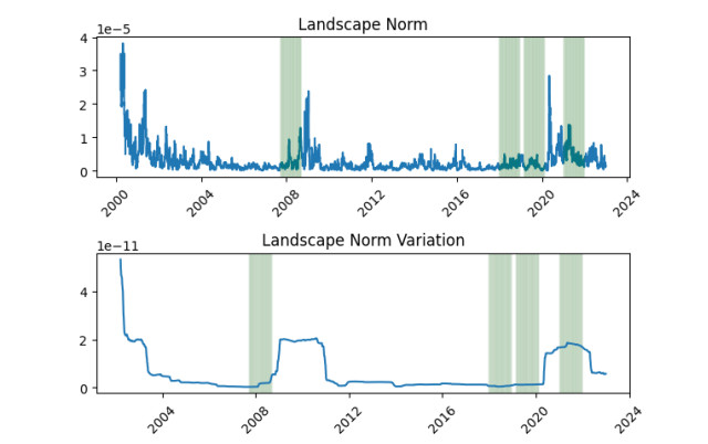
We investigate market crashes and downturns through the lens of persistent homology and persistence landscape norms. Using individual stock price data from Yahoo! Finance, we find that the variation in the persistence landscape norm as well as other measures of persistence exhibit a marked increase followed by a decline prior to historic incidents. We show that basic descriptions of persistent homology may be useful in addition to more sophisticated tools like the persistence landscape norm.
Citation: Aaron D Valdivia. Topological variability in financial markets[J]. Quantitative Finance and Economics, 2023, 7(3): 391-402. doi: 10.3934/QFE.2023019
We investigate market crashes and downturns through the lens of persistent homology and persistence landscape norms. Using individual stock price data from Yahoo! Finance, we find that the variation in the persistence landscape norm as well as other measures of persistence exhibit a marked increase followed by a decline prior to historic incidents. We show that basic descriptions of persistent homology may be useful in addition to more sophisticated tools like the persistence landscape norm.

| [1] | Bubenik P (2015) Statistical topological data analysis using persistence landscapes. J Mach Learn Res 16: 77–102. |
| [2] | Carlsson G (2009) Topology and data. Bull Am Math Soc 46. |
| [3] |
Gidea M, Katz Y(2018) Topological data analysis of financial time series: Landscapes of crashes. Physica A 491: 820–834. https://doi.org/10.1016/j.physa.2017.09.028. doi: 10.1016/j.physa.2017.09.028

|
| [4] |
Bascompte J, Brock W, Scheffer M, et al. (2009) Early-warning signals for critical transitions. Nature 461: 53–59. https://doi.org/10.1038/nature08227 doi: 10.1038/nature08227
|
| [5] |
Guttal V, Raghavendra S, Goel N, et al. (2016) Lack of critical slowing down suggests that financial meltdowns are not critical transitions, yet rising variability could signal systemic risk. PL0S ONE 11: e0144198. https://doi.org/10.1371/journal.pone.0144198 doi: 10.1371/journal.pone.0144198
|
| [6] |
Yen PTW, Cheong SA (2021) Using topological data analysis (tda) and persistent homology to analyze the stock markets in Singapore and Taiwan. Front Physics. https://doi.org/10.3389/fphy.2021.572216 doi: 10.3389/fphy.2021.572216
|
| [7] |
Antonakakis N, Cunado J, Filis G, et al. (2018) Oil volatility, oil and gas firms and portfolio diversification. Energ Econ 70: 499–515. https://doi.org/10.1016/j.eneco.2018.01.023 doi: 10.1016/j.eneco.2018.01.023
|
| [8] |
Edwards S, Biscarri JG, De Gracia FP (2003) Stock market cycles, financial liberalization and volatility. J Int Money Financ 22: 925–955. https://doi.org/10.1016/j.jimonfin.2003.09.011 doi: 10.1016/j.jimonfin.2003.09.011
|
| [9] |
Hsieh DA (1995) Nonlinear Dynamics in Financial Markets: Evidence and Implications. Financ Analy J 51: 55–62. https://doi.org/10.2469/faj.v51.n4.1921 doi: 10.2469/faj.v51.n4.1921
|


Figures(7)

Aaron D Valdivia. Topological variability in financial markets[J]. Quantitative Finance and Economics, 2023, 7(3): 391-402. doi: 10.3934/QFE.2023019


 DownLoad: