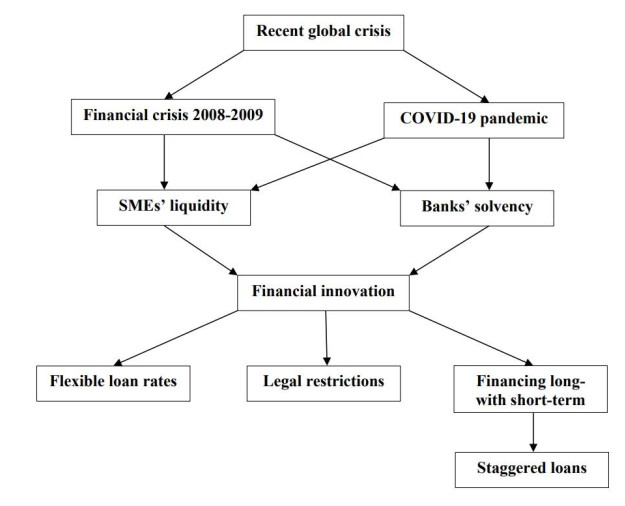
Context: The context of this paper is the unprecedented global situation which has been and is still experiencing all countries all over the world, due to the pandemic caused by Covid-19 and its variants. Apart from the important problem of health population, all countries are facing a sharp reduction in their main economic indicators: stock indices, GDP (Gross Domestic Product), rates of employment, closing down of businesses, etc. Results: In this paper, we have presented and mathematically analyzed the so-called staggered loans as a useful tool for SMEs to be applied after times of crisis. Moreover, their pros and cons, and the advantages for lenders and borrowers have been highlighted. Specifically, this kind of loan can help solve the problem of the scarce offer of credit due to monetary politics currently addressed to reduce inflation. Policy implications: Taking into account that this economic situation cannot continue for longtime, many countries are thinking about the next stages of the way-out from the crisis in all sectors of affected economies. Purpose: In this research, we seek to provide some information on the characteristics of the so-called staggered loans and the repayment system applied by some microfinance institutions in Latin America. This can help SMEs to obtain the liquidity necessary to reopen and develop their activity. Methods: Methodologically, we have presented risk-based measures able to guarantee the profitability of lenders and control the solvency of lenders and borrowers.
Citation: Salvador Cruz Rambaud, Joaquín López Pascual, Emilio M. Santandreu. Staggered loans: A flexible modality of long-term financing for SMEs in global health emergencies[J]. Quantitative Finance and Economics, 2022, 6(4): 553-569. doi: 10.3934/QFE.2022024
Context: The context of this paper is the unprecedented global situation which has been and is still experiencing all countries all over the world, due to the pandemic caused by Covid-19 and its variants. Apart from the important problem of health population, all countries are facing a sharp reduction in their main economic indicators: stock indices, GDP (Gross Domestic Product), rates of employment, closing down of businesses, etc. Results: In this paper, we have presented and mathematically analyzed the so-called staggered loans as a useful tool for SMEs to be applied after times of crisis. Moreover, their pros and cons, and the advantages for lenders and borrowers have been highlighted. Specifically, this kind of loan can help solve the problem of the scarce offer of credit due to monetary politics currently addressed to reduce inflation. Policy implications: Taking into account that this economic situation cannot continue for longtime, many countries are thinking about the next stages of the way-out from the crisis in all sectors of affected economies. Purpose: In this research, we seek to provide some information on the characteristics of the so-called staggered loans and the repayment system applied by some microfinance institutions in Latin America. This can help SMEs to obtain the liquidity necessary to reopen and develop their activity. Methods: Methodologically, we have presented risk-based measures able to guarantee the profitability of lenders and control the solvency of lenders and borrowers.

| [1] |
Acharya VV, Gale D, Yorulmazer T (2011) Rollover risk and market freezes. J Financ 66: 1177–1209. https://doi.org/10.1111/j.1540-6261.2011.01669.x doi: 10.1111/j.1540-6261.2011.01669.x

|
| [2] |
Almeida H (2021) Liquidity management during the COVID-19 pandemic. Asia-Pac J Financ Stud 50: 7–24. https://doi.org/10.1111/ajfs.12322 doi: 10.1111/ajfs.12322
|
| [3] |
Bartik A, Bertrand M, Cullen Z, et al. (2020) The impact of COVID-19 on small business outcomes and expectations. Proc Natl Acad Sci 117: 17656–17666. https://doi.org/10.1073/pnas.200699111 doi: 10.1073/pnas.200699111
|
| [4] |
Berger AN, Udell GF (1992) Some evidence on the empirical significance of credit rationing. J Polit Econ 100: 1047–1077. https://doi.org/10.1086/261851 doi: 10.1086/261851
|
| [5] | Brockmann D, Helbing D (2013) The hidden geometry of complex, network-driven contagion phenomena. Science 342: 1337–1342. https://www.science.org/doi/10.1126/science.1245200 |
| [6] |
Burns C, Clifton J, Quaglia L (2018) Explaining policy change in the EU: Financial reform after the crisis. J Eur Public Policy 25: 728–746. https://doi.org/10.1080/13501763.2017.1301535 doi: 10.1080/13501763.2017.1301535
|
| [7] |
Cao S, Leung D (2020) Credit constraints and productivity of SMEs: Evidence from Canada. Econ Model 88: 163–180. https://doi.org/10.1016/j.econmod.2019.09.018 doi: 10.1016/j.econmod.2019.09.018
|
| [8] |
Centeno MA, Nag M, Patterson TS, Shaver, et al. (2015) The emergence of global systemic risk. Annu Rev Sociol 41: 65–85. https://doi.org/10.1146/annurev-soc-073014-112317 doi: 10.1146/annurev-soc-073014-112317
|
| [9] | Cruz Rambaud S, Valls Martínez MC (2014) Introducción a las Matemáticas Financieras. |
| [10] |
Cruz Rambaud S, Sánchez Pérez AM (2018) A deforming time approach to the treatment of risk in projects evaluation. J Risk Financ 19: 548–563. https://doi.org/10.1108/JRF-11-2017-0175 doi: 10.1108/JRF-11-2017-0175
|
| [11] |
Del Giudice A (2017) Impact of the Market in Financial Instruments Directive (MiFID) on the Italian financial market: Evidence from bank bonds. J Bank Regul 18: 256–267. https://doi.org/10.1057/s41261-016-0035-7 doi: 10.1057/s41261-016-0035-7
|
| [12] |
Demma C (2017) Credit scoring and the quality of business credit during the crisis. Econ Notes 46: 269–306. https://doi.org/10.1111/ecno.12080 doi: 10.1111/ecno.12080
|
| [13] |
Gasper D (2019) The road to the sustainable development goals: Building global alliances and norms. J Global Ethics 15: 118–137. https://doi.org/10.1080/17449626.2019.1639532 doi: 10.1080/17449626.2019.1639532
|
| [14] |
Diamond DW (1991) Debt maturity structure and liquidity risk. Q J Econ 106: 709–737. https://doi.org/10.2307/2937924 doi: 10.2307/2937924
|
| [15] |
Drechsler I, Drechsel T, Marques-Ibanez D, et al. (2016) Who borrows from the lender of last resort? J Financ 71: 1933–1974. https://doi.org/10.1111/jofi.12421 doi: 10.1111/jofi.12421
|
| [16] |
Fabris N (2022) Impact of COVID-19 pandemic on financial innovation, cashless society, and cyber risk. ECONOMICS 10: 73–86. https://doi.org/10.2478/eoik-2022-0002 doi: 10.2478/eoik-2022-0002
|
| [17] | Flores PP, Fullerton TM, Olivas AC (2007) Evidencia empírica sobre deuda externa, inversión y crecimiento en México, 1980–2003. Análisis Económico 50: 149–171. |
| [18] |
Fujiwara I, Teranishi Y (2017) Financial frictions and policy cooperation: A case with monopolistic banking and staggered loan contracts. J Int Econ 104: 19–43. https://doi.org/10.1016/j.jinteco.2016.09.004 doi: 10.1016/j.jinteco.2016.09.004
|
| [19] |
Giones F, Brem A, Pollack JM, et al. (2020) Revising entrepreneurial action in response to exogenous shocks: Considering the COVID-19 pandemic. J Bus Venturing Insights 14: e00186. https://doi.org/10.1016/j.jbvi.2020.e00186 doi: 10.1016/j.jbvi.2020.e00186
|
| [20] | Greenwald DL, Krainer J, Paul P (2020) The Credit Line Channel. Federal Reserve Bank of San Francisco Working Paper 2020-26. https://doi.org/10.24148/wp2020-26 |
| [21] | Harel R (2021) The impact of COVID-19 on small businesses' performance and innovation. Glob Bus Rev. https://doi.org/10.1177/09721509211039145 |
| [22] | International Monetary Fund (2020) Enhancing the emergency financing toolkit-Responding to the COVID-19 pandemic. |
| [23] | Jasova M, Mendicino C, Supera D (2018) Rollover risk and bank lending behavior: Evidence from unconventional central bank liquidity. Available from: https://economicdynamics.org/meetpapers/2018/paper_500.pdf. |
| [24] | Kalemli-Ozcan S, Laeven L, Moreno D (2019) Debt overhang, rollover risk, and corporate investment: evidence from the European crisis. European Central Bank. Working Paper Series 2241. http://dx.doi.org/10.2139/ssrn.3336457 |
| [25] |
Klein VB, Todesco JL (2021) COVID-19 crisis and SMEs responses: The role of digital transformation. Knowl Process Manag 28: 117–133. https://doi.org/10.1002/kpm.1660 doi: 10.1002/kpm.1660
|
| [26] |
Kurt H, Peng X (2021) Does corporate social performance lead to better financial performance? Evidence from Turkey. Green Financ 3: 464–482. https://doi.org/10.3934/GF.2021021 doi: 10.3934/GF.2021021
|
| [27] | López Pascual J, Sebastián González A (2015) Economía y Gestión Bancaria. Ediciones Pirámide, S.A.: Madrid (Spain). |
| [28] | Microtracker (2019) Industry data. Available from: https://microtracker.org/explore/industry-data/. |
| [29] | Mills CK, Battisto J, Lieberman S, et al. (2018) Latino-owned businesses. Shining a light on national trends. Interise, Stanford Latino Entrepreneurship Initiative. The Federal Reserve Bank, New York. |
| [30] |
Prorokowski L (2015) MiFID II compliance - are we ready? J Financ Regul Compl 23: 196–206. https://doi.org/10.1108/JFRC-02-2014-0009 doi: 10.1108/JFRC-02-2014-0009
|
| [31] |
Santandreu EM, López Pascual J (2019) Microfinance institutions in the USA: The glocalization of microcredit policies in relation to gender. Enterp Dev Microfinance 30: 73–96. https://doi.org/10.3362/1755-1986.18-00019 doi: 10.3362/1755-1986.18-00019
|
| [32] |
Santandreu EM, López Pascual J, Cruz Rambaud S (2020) Determinants of repayment among male and female microcredit clients in the USA. An approach based on managers' perceptions. Sustainability 12: 1701. https://doi.org/10.3390/su12051701 doi: 10.3390/su12051701
|
| [33] |
Tang J, Zhang SX, Lin S (2021) To reopen or not to reopen? How entrepreneurial alertness influences small business reopening after the COVID-19 lockdown. J Bus Venturing Insights 16: e00275. https://doi.org/10.1016/j.jbvi.2021.e00275 doi: 10.1016/j.jbvi.2021.e00275
|
| [34] |
Teranishi Y (2015) Smoothed interest rate setting by central banks and staggered loan contracts. Econ J 125: 162–183. https://doi.org/10.1111/ecoj.12092 doi: 10.1111/ecoj.12092
|
| [35] |
Wolfe MT, Patel PC (2021) Everybody hurts: Self-employment, financial concerns, mental distress, and well-being during COVID-19. J Bus Venturing Insights 15: e00231. https://doi.org/10.1016/j.jbvi.2021.e00231 doi: 10.1016/j.jbvi.2021.e00231
|
| [36] |
Xu M, Albitar K, Li Z (2020) Does corporate financialization affect EVA? Early evidence from China. Green Financ 2: 392–408. https://doi.org/10.3934/GF.2020021 doi: 10.3934/GF.2020021
|


Figures(3) / Tables(3)

Salvador Cruz Rambaud, Joaquín López Pascual, Emilio M. Santandreu. Staggered loans: A flexible modality of long-term financing for SMEs in global health emergencies[J]. Quantitative Finance and Economics, 2022, 6(4): 553-569. doi: 10.3934/QFE.2022024


 DownLoad: