A comprehensive high pure momentum equity timing framework using the Kalman filter and ARIMA forecasting

Tsumbedzo Mashamba; Modisane Seitshiro; Isaac Takaidza; Tsumbedzo Mashamba; Modisane Seitshiro; Isaac Takaidza

doi:10.3934/DSFE.2024023

Data Science in Finance and Economics

2024, Volume 4, Issue 4: 548-569. doi: 10.3934/DSFE.2024023

Previous Article Next Article

Research article

A comprehensive high pure momentum equity timing framework using the Kalman filter and ARIMA forecasting

1.
School of Mathematical and Statistical Sciences, North-West University, Hendrik Van Eck Boulevard, Vanderbijlpark, 1900, South Africa
2.
Centre for Business Mathematics and Informatics, North-West University, Potchefstroom, 2531, South Africa
3.
National Institute of Theorectical and Computational Sciences (NITheCS), Stellenbosch, South Africa

Received: 28 June 2024 Revised: 30 October 2024 Accepted: 27 November 2024 Published: 29 November 2024
JEL Codes: G11, G12, G17, C22

The pursuit of higher returns has led to a growing interest in factor timing as a strategy to enhance portfolio returns. Momentum is a popular factor, which involves buying securities that have shown consistent price appreciation over the past 3 to 12 months or past few years, with the expectation that the trend will continue and reducing exposure to those that consistently declined. An important part of a factor timing strategy is in the portfolio optimization process. This article aimed to first construct a large capitalization pure momentum portfolio, which included a dynamic stringent portfolio construction process criteria for selecting stocks estimated from historical data. Second, as a part of the portfolio's risk management strategy, the Kalman filter was applied to the historical performance of this portfolio. Lastly, the ARIMA forecast was used to estimate expected performance and the confidence intervals. The empirical results showed that this pure equity momentum factor timing framework with the Kalman filter together with the ARIMA (autoregressive integrated moving average) forecasting methodology was iterative and incorporated new information as it became available and further enhanced the monitoring and rebalancing process. This adaptive approach enabled the portfolio to capitalize on time-varying return anomalies as they occured.
- momentum,
- factor timing,
- Kalman filter,
- return predictability,
- factor investing,
- investment style factors
Citation: Tsumbedzo Mashamba, Modisane Seitshiro, Isaac Takaidza. A comprehensive high pure momentum equity timing framework using the Kalman filter and ARIMA forecasting[J]. Data Science in Finance and Economics, 2024, 4(4): 548-569. doi: 10.3934/DSFE.2024023

Related Papers:

Abstract

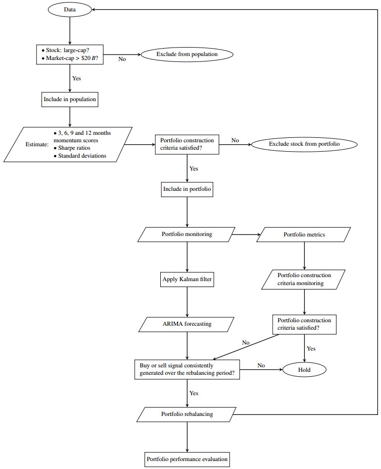
The pursuit of higher returns has led to a growing interest in factor timing as a strategy to enhance portfolio returns. Momentum is a popular factor, which involves buying securities that have shown consistent price appreciation over the past 3 to 12 months or past few years, with the expectation that the trend will continue and reducing exposure to those that consistently declined. An important part of a factor timing strategy is in the portfolio optimization process. This article aimed to first construct a large capitalization pure momentum portfolio, which included a dynamic stringent portfolio construction process criteria for selecting stocks estimated from historical data. Second, as a part of the portfolio's risk management strategy, the Kalman filter was applied to the historical performance of this portfolio. Lastly, the ARIMA forecast was used to estimate expected performance and the confidence intervals. The empirical results showed that this pure equity momentum factor timing framework with the Kalman filter together with the ARIMA (autoregressive integrated moving average) forecasting methodology was iterative and incorporated new information as it became available and further enhanced the monitoring and rebalancing process. This adaptive approach enabled the portfolio to capitalize on time-varying return anomalies as they occured.

References

[1]	Aked M (2021) Factor Timing: Keep It Simple. Research Affiliates.
[2]	Aiken AL, Kang M (2023) Hedge fund manager timing and selectivity skill over time, A holdings-based estimate. Financ Res Lett 58.
[3]	Aggarwal D (2022) Defining and measuring market sentiments: a review of the literature. Qual Res Financ Mark 14: 270-288. https://doi.org/10.1108/QRFM-03-2018-0033 doi: 10.1108/QRFM-03-2018-0033
[4]	Asness C, Chandra S, Ilmanen A, et al. (2018) Contrarian Factor Timing Is Deceptively Difficult. J Portfoli Manage Forthcoming 43.
[5]	Asness C, Ilmanen A, Maloney T (2017) Market Timing: Sin a Little, Resolving the Valuation Timing Puzzle. J Invest Manag 15: 23–40.
[6]	Carhart MM (1997) On Persistence in Mutual Fund Performance. J Financ 52: 57-82.
[7]	Chin A, Gupta P (2020) Timing is Not Everything—Assessing Manager Skill in Factor Timing. J Invest Manage 18: 34-51.
[8]	Clare A, Sherman M, O'Sullivan N, et al. (2022) Manager characteristics: Predicting fund performance. Int Rev Financ Anal 80: 102049. https://doi.org/10.1016/j.irfa.2022.102049 doi: 10.1016/j.irfa.2022.102049
[9]	Daniel K, Grinblatt M, Titman S, et al. (1997) Measuring Mutual Fund Performance with Characteristic-Based Benchmarks. J Financ 52: 1035-1058. https://doi.org/10.1111/j.1540-6261.1997.tb02724.x doi: 10.1111/j.1540-6261.1997.tb02724.x
[10]	Davies J, Gibbon D, Shores S, et al. (2019) Implementation Matters: Relaxing Constraints Can Improve the Potential Returns of Factor Strategies. J Portfoli Manage Quant 45: 101-114. https://doi.org/10.3905/jpm.2019.45.3.101 doi: 10.3905/jpm.2019.45.3.101
[11]	Dichtl H, Drobetz W, Lohre H, et al. (2019) Optimal Timing and Tilting of Equity Factors. Financ Anal J 75: 84-102. https://doi.org/10.1080/0015198X.2019.1645478 doi: 10.1080/0015198X.2019.1645478
[12]	Drew ME, Veeraraghavan M, Wilson V (2005) Market Timing, Selectivity and Alpha Generation: Evidence from Australian Equity Superannuation Funds. Invest Manage Financ Innov 2: 111-127.
[13]	Fama EF, French KR (1992) The cross-section of expected stock returns. J Financ 47: 427-465.
[14]	Fergis K, Gallagher K, Hodges P, et al. (2019) Defensive Factor Timing. J Portfoli Manage Quant 45: 50-68. https://doi.org/10.3905/jpm.2019.45.3.050 doi: 10.3905/jpm.2019.45.3.050
[15]	Fischer AM, Greminger RP, Grisse C, et al. (2021) Portfolio rebalancing in times of stress. J Int Money Financ 113. https://doi.org/10.1016/j.jimonfin.2021.102360 doi: 10.1016/j.jimonfin.2021.102360
[16]	Galati L (2024) Exchange market share, market makers, and murky behavior: The impact of no-fee trading on cryptocurrency market quality. J Bank Financ 165.https://doi.org/10.1016/j.jbankfin.2024.107222 doi: 10.1016/j.jbankfin.2024.107222
[17]	George TJ, Hwang C (2004) The 52-Week High and Momentum Investing. J Financ 59: 2145-2176. https://doi.org/10.1111/j.1540-6261.2004.00695.x doi: 10.1111/j.1540-6261.2004.00695.x
[18]	Gupta T, Kelly B (2019) Factor Momentum Everywhere. J Portfoli Manage Quant 45: 13-36. https://doi.org/10.3905/jpm.2019.45.3.013 doi: 10.3905/jpm.2019.45.3.013
[19]	Huang J, Zhang P, Zhang J (2024) Understanding Momentum and Reversal Investing Strategies. J Econ Financ Account Stud 5: 106-112. https://doi.org/10.32996/jefas.2023.5.1.8 doi: 10.32996/jefas.2023.5.1.8
[20]	Huberman G, Wang Z (2005) Arbitrage Pricing Theory. Federal Reserve Bank of New York Staff Reports. Available from: https://www.econstor.eu/handle/10419/60653.
[21]	Hong H, Stein JC (1999) A Unified Theory of Underreaction, momentum trading, and overreaction in Asset markets. J Financ 54: 2143-2184. https://doi.org/10.1111/0022-1082.00184 doi: 10.1111/0022-1082.00184
[22]	Isaenko S (2023) Transaction costs, frequent trading, and stock prices. J Financ Mark 64: 100775. https://doi.org/10.1016/j.finmar.2022.100775 doi: 10.1016/j.finmar.2022.100775
[23]	Jegadeesh N, Titman S (1993) Returns to buying winners and selling losers: Implications for stock market efficiency. J Financ 48: 65-91.
[24]	Kálmán RE (1960) A New Approach to Linear Filtering and Prediction Problems. J Basic Eng 82: 35-45. https://doi.org/10.1115/1.3662552 doi: 10.1115/1.3662552
[25]	Karki D, Khadka PB (2023) Momentum Investment Strategies across Time and Trends: A Review and Preview. Nepal J Multidiscip Res 7: 62-83. https://ssrn.com/abstract = 4837507
[26]	Keisler J, Linkov I (2011) Managing a portfolio of risks. Management Science and Information Systems Faculty Publication Series, 33.
[27]	Kimball MS, Shapiro MD, Shumway T, et al. (2020) Portfolio rebalancing in general equilibrium. J Financ Econ 135: 816-834. https://doi.org/10.3386/w24722 doi: 10.3386/w24722
[28]	Kwon D (2022) Dynamic Factor Rotation Strategy: A Business Cycle Approach. Int J Financ Stud 10: 46. https://doi.org/10.3390/ijfs10020046 doi: 10.3390/ijfs10020046
[29]	Lintner J (1965) The Valuation of Risk Assets and the Selection of Risky Investments in Stock Portfolios and Capital Budgets. Rev Econ Stat 47: 13-37.
[30]	Markowitz H (1952) Portfolio Selection. J Financ 7: 77-91.
[31]	Moskowitz TJ, Grinblatt M (1999) Do industries explain momentum? J Financ 54: 1249-1290.
[32]	Osinga B, Schauten M, Zwinkels RCJ (2020) Timing is Money: The Factor Timing Ability of Hedge Fund Managers. Available at SSRN, 2811163.
[33]	Plastira S (2014) Performance evaluation of size, book-to-market and momentum portfolios. Procedia Econ Financ 14: 481-490. https://doi.org/10.1016/S2212-5671(14)00737-0 doi: 10.1016/S2212-5671(14)00737-0
[34]	Ross SA (1976) The Arbitrage Theory of Asset Pricing. J Econ Theory 13: 341-360.
[35]	Sharpe WF (1964) Capital asset prices: A theory of market equilibrium under conditions of risk. J Financ 19: 425-442
[36]	Shumway RH, Stoffer DS (2017) Time Series Analysis and Its Applications: With R Examples (4th ed.). Springer.
[37]	Souza TO (2020) Macro-Finance and Factor Timing: Time-Varying Factor Risk and Price of Risk Premiums. Available at SSRN.
[38]	Treynor J, Mazuy K (1966) Can Mutual Funds Outguess the Market? Harvard Bus Rev 44: 131-136.
[39]	Wang N, Siu TK (2024) Investment-consumption optimization with transaction cost and learning about return predictability. Eur J Oper Res 318: 877-891. https://doi.org/10.1016/j.ejor.2024.06.024 doi: 10.1016/j.ejor.2024.06.024
[40]	Zheng Y, Osmer E, Zu D (2024) Timing sentiment with style: Evidence from mutual funds. J Bank Financ 164. https://doi.org/10.1016/j.jbankfin.2024.107197 doi: 10.1016/j.jbankfin.2024.107197

Reader Comments

Your name:*

Email:*
© 2024 the Author(s), licensee AIMS Press. This is an open access article distributed under the terms of the Creative Commons Attribution License (http://creativecommons.org/licenses/by/4.0)