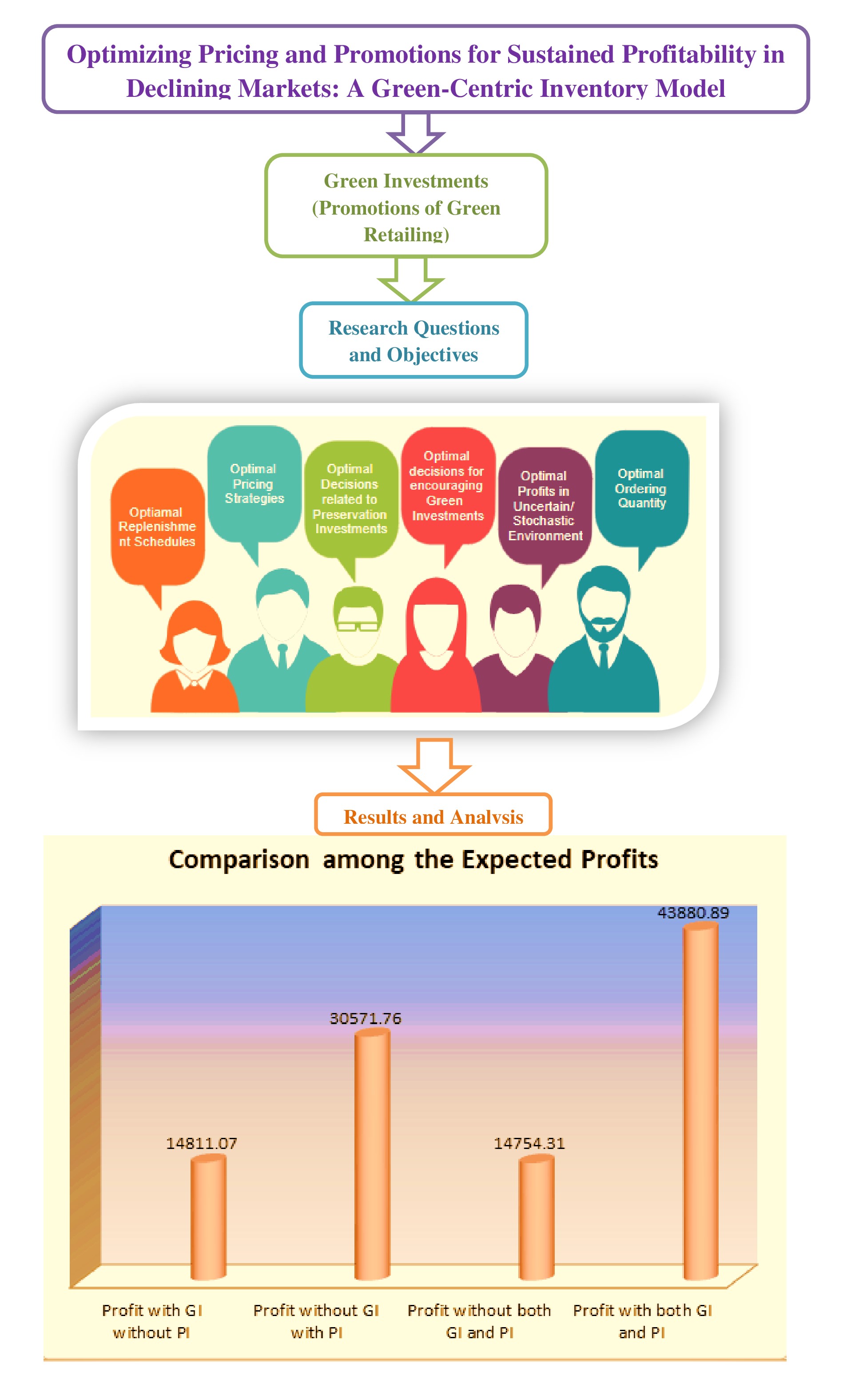
In the face of a competitive and ever-changing business landscape, companies often grapple with the challenge of sustaining their products in declining markets. To combat this issue, effective strategies such as promotional efforts play a pivotal role in boosting demand and maintaining market position. Additionally, businesses are increasingly focusing on ecological safety and greening efforts to minimize their environmental impact while ensuring the production of environmentally friendly products. These green initiatives not only contribute to environmental sustainability but can also enhance retailer profitability. This article presents an innovative inventory model tailored for perishable products within a stochastic environment. The model integrates elements such as linear pricing, time dynamics, promotional efforts, and a demand rate that depends non-linearly on the level of greening efforts. The model also considers partial backlogging of shortages, lost sales, time-dependent product deterioration, and investments in preservation technology to mitigate deterioration effects. The primary objective is to calculate the retailer's profit function, taking into account cycle time, selling price, promotional effort, and greening effort as key variables. To address this complex problem, the article introduces an algorithm for finding feasible solutions. Furthermore, the concavity of these solutions is demonstrated through graphical analysis. A numerical example is provided to illustrate the application of the model, and sensitivity analysis is conducted to elucidate how changes in inventory parameters impact decision variables. We will also depicted the short representation of proposed study in
Citation: Mamta Keswani, Uttam Khedlekar. 2024: Optimizing pricing and promotions for sustained profitability in declining markets: A Green-Centric inventory model, Data Science in Finance and Economics, 4(1): 83-131. doi: 10.3934/DSFE.2024004
In the face of a competitive and ever-changing business landscape, companies often grapple with the challenge of sustaining their products in declining markets. To combat this issue, effective strategies such as promotional efforts play a pivotal role in boosting demand and maintaining market position. Additionally, businesses are increasingly focusing on ecological safety and greening efforts to minimize their environmental impact while ensuring the production of environmentally friendly products. These green initiatives not only contribute to environmental sustainability but can also enhance retailer profitability. This article presents an innovative inventory model tailored for perishable products within a stochastic environment. The model integrates elements such as linear pricing, time dynamics, promotional efforts, and a demand rate that depends non-linearly on the level of greening efforts. The model also considers partial backlogging of shortages, lost sales, time-dependent product deterioration, and investments in preservation technology to mitigate deterioration effects. The primary objective is to calculate the retailer's profit function, taking into account cycle time, selling price, promotional effort, and greening effort as key variables. To address this complex problem, the article introduces an algorithm for finding feasible solutions. Furthermore, the concavity of these solutions is demonstrated through graphical analysis. A numerical example is provided to illustrate the application of the model, and sensitivity analysis is conducted to elucidate how changes in inventory parameters impact decision variables. We will also depicted the short representation of proposed study in

| [1] |
Abad P (1996) Optimal pricing and lot-sizing under conditions of perishability and partial backordering, Manag Sci 42: 1093–1104. https://doi.org/10.1287/mnsc.42.8.1093 doi: 10.1287/mnsc.42.8.1093

|
| [2] | Abad P (2001) Optimal price and order size for a reseller under partial backordering. Comput Oper Res 28: 53–65. |
| [3] |
Abdul Hakim M, Hezam I, Alrasheedi A, et al. (2022) Pricing policy in an inventory model with green level dependent demand for a deteriorating item. Sustainability 14: 4646. https://doi.org/10.3390/su14084646 doi: 10.3390/su14084646
|
| [4] |
Chang C, Teng J, Goyal S (2010) Optimal replenishment policies for non-instantaneous deteriorating items with stock-dependent demand. Int J Prod Eco 123: 62–68. https://doi.org/10.1016/j.ijpe.2009.06.042 doi: 10.1016/j.ijpe.2009.06.042
|
| [5] |
Chang C, Teng J, Goyal S (2015) Optimal pricing and ordering policies for non-instantaneously deteriorating items under order-size-dependent delay in payments. Appl Math Model 39: 747–763. https://doi.org/10.1016/j.apm.2014.07.002 doi: 10.1016/j.apm.2014.07.002
|
| [6] |
Chen Z, Chen C, Bidanda B, et al. (2017) Optimal inventory replenishment, production, and promotion effect with risks of production disruption and stochastic demand. J Ind Prod Eng 34: 79–89. https://doi.org/10.1080/21681015.2016.1233912 doi: 10.1080/21681015.2016.1233912
|
| [7] |
Chkanikova O, Lehner M (2015) Private eco-brands and green market development: towards new forms of sustainability governance in the food retailing. J Clean Prod 107: 74–84. https://doi.org/10.1016/j.jclepro.2014.05.055 doi: 10.1016/j.jclepro.2014.05.055
|
| [8] |
Dada M, Petruzzi N, Schwarz L (2007). A newsvendor's procurement problem when suppliers are unreliable. Manuf Serv Oper Manag 9: 9–32. https://doi.org/10.1287/msom.1060.0128 doi: 10.1287/msom.1060.0128
|
| [9] |
Dash B, Pattnaik M, Pattnaik H (2014) The impact of promotional activities and inflationary trends on a deteriorated inventory model allowing delay in payment. J Bus Manag Sci 2: 1–16. https://doi.org/10.12691/jbms-2-3A-1 doi: 10.12691/jbms-2-3A-1
|
| [10] |
De SK, Sana S (2013) Backlogging EOQ model for promotional effort and selling price sensitive demand - an intuitionistic fuzzy approach. Ann Oper Res 233: 57–76. https://doi.org/10.1007/s10479-013-1476-3 doi: 10.1007/s10479-013-1476-3
|
| [11] |
Dye C (2007) Joint pricing and ordering policy for a deteriorating inventory with partial backlogging. Omega 35: 184–189. https://doi.org/10.1016/j.omega.2005.05.002 doi: 10.1016/j.omega.2005.05.002
|
| [12] |
Ghosh D, Shah J (2012) A comparative analysis of greening policies across supply chain structures. Int J Prod Econ 135: 568–583. https://doi.org/10.1016/j.ijpe.2011.05.027 doi: 10.1016/j.ijpe.2011.05.027
|
| [13] |
Hakim IM, Alrasheedi AF, Gwak J (2022) Pricing policy in an inventory model with green level dependent demand for a deteriorating item. Sustainability 14: 4646. https://doi.org/10.3390/su14084646 doi: 10.3390/su14084646
|
| [14] |
He Y, Zhao X, Zhao L, et al. (2009) Coordinating a supply chain with effort and price dependent stochastic demand. Appl Math Model 33: 2777–2790. https://doi.org/10.1016/j.apm.2008.08.016 doi: 10.1016/j.apm.2008.08.016
|
| [15] |
Hollier R, Mak K (1983) Inventory replenishment policies for deteriorating items in a decline market. Int J Prod Res 21: 813–826. https://doi.org/10.1080/00207548308942414 doi: 10.1080/00207548308942414
|
| [16] |
Jaggi C, Sharma A, Tiwari S (2015) Credit financing in economic ordering policies for non-instantaneous deteriorating items with price dependent demand under permissible delay in payments: A new approach. Int J Ind Eng Comput 6: 481–502. https://doi.org/10.5267/j.ijiec.2015.5.003 doi: 10.5267/j.ijiec.2015.5.003
|
| [17] |
Jauhari WA, Wangsa ID, Hishamuddin H, et al. (2023) A sustainable vendor-buyer inventory model with incentives, green investment and energy usage under stochastic demand. Cogent Bus Manag 10: 2158609. https://doi.org/10.1080/23311975.2022.2158609 doi: 10.1080/23311975.2022.2158609
|
| [18] |
Jones P, Hillier D, Comfort D (2011) Shopping for tomorrow: promoting sustainable consumption within food stores. Br Food J 113: 935–948. https://doi.org/10.1108/00070701111148441 doi: 10.1108/00070701111148441
|
| [19] |
Khedlekar UK, Kumar L, Keswani M, et al. (2023) A stochastic inventory model with price-sensitive demand, restricted shortage and promotional efforts. Yugosl J Oper Res 33. http://dx.doi.org/10.2298/YJOR220915010K doi: 10.2298/YJOR220915010K
|
| [20] |
Kumar P (2014) Greening retail: an Indian experience. Int J Retail Distrib Manag 42: 613–625. https://doi.org/10.1108/IJRDM-02-2013-0042 doi: 10.1108/IJRDM-02-2013-0042
|
| [21] |
Lai K, Cheng T, Tang A, et al. (2010) Green retailing: Factors for success. Calif Manag Rev 52: 6–31. https://doi.org/10.1525/cmr.2010.52.2.6. doi: 10.1525/cmr.2010.52.2.6
|
| [22] |
Li G, He X, Zhou J, et al. (2019) Pricing, replenishment and preservation technology investment decisions for non-instantaneous deteriorating items. Omega 84: 114–126. https://doi.org/10.1016/j.omega.2018.05.001 doi: 10.1016/j.omega.2018.05.001
|
| [23] |
Li X, Zhu G(2023) Green supply chain coordination considering carbon emissions and product green level dependent demand. Mathematics 11: 2355. https://doi.org/10.3390/math11102355 doi: 10.3390/math11102355
|
| [24] |
Maihami R, Kamalabadi I (2012) Joint pricing and inventory control for non-instantaneous deteriorating items with partial backlogging and time and price dependent demand. Int J Prod Econ 136: 116–122. https://doi.org/10.1016/j.ijpe.2011.09.020 doi: 10.1016/j.ijpe.2011.09.020
|
| [25] |
Maihami R, Karimi B (2014) Optimizing the pricing and replenishment policy for non-instantaneous deteriorating items with stochastic demand and promotional efforts. Comput Oper Res 51: 302–312. https://doi.org/10.1016/j.cor.2014.05.022 doi: 10.1016/j.cor.2014.05.022
|
| [26] |
Manna AK, Bhunia AK (2022) Investigation of green production inventory problem with selling price and green level sensitive interval-valued demand via different metaheuristic algorithms. Soft Computing 26: 10409–10421. https://doi.org/10.1007/s00500-022-06856-9 doi: 10.1007/s00500-022-06856-9
|
| [27] |
Mishra V, Singh L (2011) Deteriorating inventory model for time dependent demand and holding cost with partial backlogging. Int J Manag 6: 267–271. https://doi.org/10.1080/17509653.2011.10671172 doi: 10.1080/17509653.2011.10671172
|
| [28] |
Mondal C, Giri B (2020) Pricing and used product collection strategies in a two-period closed-loop supply chain under greening level and effort dependent demand. J Clean Prod 265: 121335. https://doi.org/10.1016/j.jclepro.2020.121335 doi: 10.1016/j.jclepro.2020.121335
|
| [29] |
Nath BK, Sen N (2021) A Completely backlogged two-warehouse inventory model for non-instantaneous deteriorating items with time and selling price dependent demand. Int J Appl Comput Math 7: 145. https://doi.org/10.1007/s40819-021-01070-x doi: 10.1007/s40819-021-01070-x
|
| [30] |
Nouira I, Frein Y, Hadj-Alouane AB (2014) Optimization of manufacturing systems under environmental considerations for a greenness-dependent demand. Int J Prod Econ 150: 188–198. https://doi.org/10.1016/j.ijpe.2013.12.024 doi: 10.1016/j.ijpe.2013.12.024
|
| [31] | Ouyang L, Chen C, Chang H (2002) Quality improvement, set-up cost and lead-time reductions in lot size reorder point models with an imperfect production process. Comput Oper Res 29: 1701–1717. |
| [32] |
Pakhira N, Maiti M, Maiti M (2017) Two-level supply chain of a seasonal deteriorating item with time, price, and promotional cost dependent demand under finite time horizon. Am J Math Manag Sci 36: 292–315. https://doi.org/10.1080/01966324.2017.1334605 doi: 10.1080/01966324.2017.1334605
|
| [33] | Panda S, Saha S, Basu M (2013) Optimal pricing and lot-sizing for perishable inventory with price and time dependent ramp-type demand. Int J Syst Sci 44: 127–138. |
| [34] |
Panja S, Mondal S (2019) Analyzing a four-layer green supply chain imperfect production inventory model for green products under type-2 fuzzy credit period. Comput Ind Eng 129: 435–453. https://doi.org/10.1016/j.cie.2019.01.059 doi: 10.1016/j.cie.2019.01.059
|
| [35] |
Panja S, Mondal SK (2020) Exploring a two-layer green supply chain game theoretic model with credit linked demand and mark-up under revenue sharing contract. J Clean Prod 250: 119491. https://doi.org/10.1016/j.jclepro.2019.119491 doi: 10.1016/j.jclepro.2019.119491
|
| [36] |
Paul A, Garai T, Giri B (2023) Sustainable supply chain coordination with greening and promotional effort dependent demand. Int J Procure Manag 16: 196–233. https://doi.org/10.1504/IJPM.2023.128478 doi: 10.1504/IJPM.2023.128478
|
| [37] |
Rajeswari N, Vanjikkodi T (2012) An inventory model for items with two parameter Weibull distribution deterioration and backlogging. Am J Oper Res 2. https://doi.org/10.4236/ajor.2012.22029 doi: 10.4236/ajor.2012.22029
|
| [38] |
Rapolu C, Kandpal D (2020) Joint pricing, advertisement, preservation technology investment and inventory policies for non-instantaneous deteriorating items under trade credit. Opsearch 57: 274–300. https://doi.org/10.1007/s12597-019-00427-7 doi: 10.1007/s12597-019-00427-7
|
| [39] |
Rastogi M, Singh S (2019) An inventory system for varying deteriorating pharmaceutical items with price-sensitive demand and variable holding cost under partial backlogging in healthcare industries. Sadhana 44: 95. https://doi.org/10.1007/s12046-019-1075-3 doi: 10.1007/s12046-019-1075-3
|
| [40] | Rani S, Ali R, Agarwal A (2018) An optimal inventory model For deteriorating products In green supply chain under shortage. Int J Sci Adv Res Technol 4: 1371–1377. |
| [41] |
Rabbani M, Zia NP, Rafiei H (2017) Joint optimal inventory, dynamic pricing and advertisement policies for non-instantaneous deteriorating items. RAIRO - Operations Research 51: 1251–1267. https://doi.org/10.1051/ro/2016074 doi: 10.1051/ro/2016074
|
| [42] |
Saha S, Nielsen I, Moon I (2017) Optimal retailer investments in green operations and preservation technology for deteriorating items. J Clean Prod 140: 1514–1527. https://doi.org/10.1016/j.jclepro.2016.09.229 doi: 10.1016/j.jclepro.2016.09.229
|
| [43] | Saha S, Sen N (2019) An inventory model for deteriorating items with time and price dependent demand and shortages under the effect of inflation. Int J Math Sci 14: 377–388. |
| [44] |
Sana S (2010) Optimal selling price and lot size with time varying deterioration and partial backlogging. Appl Math Comput 217: 185–194. https://doi.org/10.1016/j.amc.2010.05.040 doi: 10.1016/j.amc.2010.05.040
|
| [45] |
San-José L, Sicilia J, Alcaide-López-de-Pablo D (2018) An inventory system with demand dependent on both time and price assuming backlogged shortages. Eur J Oper Res 270: 889–897. https://doi.org/10.1016/j.ejor.2017.10.042 doi: 10.1016/j.ejor.2017.10.042
|
| [46] | Shah N, Shukla K (2009) Deteriorating inventory model for waiting time partial backlogging. Int J Manag 3: 421–428. |
| [47] |
Shah N, Shah P, Patel M (2021) Retailer's inventory decisions with promotional efforts and preservation technology investments when supplier offers quantity discounts. Opsearch 58: 1116–1132. https://doi.org/10.1007/s12597-021-00516-6 doi: 10.1007/s12597-021-00516-6
|
| [48] |
Shah N, Rabari K, Patel E (2023) Greening efforts and deteriorating inventory policies for price-sensitive stock-dependent demand. Int J Syst Sci Oper 10: 2022808. https://doi.org/10.1080/23302674.2021.2022808 doi: 10.1080/23302674.2021.2022808
|
| [49] |
Shah N, Keswani M, Khedlekar UK, et al. (2023) Non-instantaneous controlled deteriorating inventory model for stock-price-advertisement dependent probabilistic demand under trade credit financing. OPSEARCH. https://doi.org/10.1007/s12597-023-00701-9 doi: 10.1007/s12597-023-00701-9
|
| [50] |
Singh S, Rathore H (2015) Optimal payment policy with preservation technology investment and shortages under trade-credit. Indian J Sci Technol 8: 1–10. https://doi.org/10.17485/ijst/2015/v8iS7/64489 doi: 10.17485/ijst/2015/v8iS7/64489
|
| [51] |
Soni H, Chauhan A (2018) Joint pricing, inventory, and preservation decisions for deteriorating items with stochastic demand and promotional efforts. J Ind Eng Int 14: 831–843. https://doi.org/10.1007/s40092-018-0265-7 doi: 10.1007/s40092-018-0265-7
|
| [52] |
Soni H, Suthar D (2019) Pricing and inventory decisions for non-instantaneous deteriorating items with price and promotional effort stochastic demand. J Control Decis 6: 191–215. https://doi.org/10.1080/23307706.2018.1478327 doi: 10.1080/23307706.2018.1478327
|
| [53] |
Tang A, Lai K, Cheng T (2016) A multi-research-method approach to studying environmental sustainability in retail operations. Int J Prod Econ 171: 394–404. https://doi.org/10.1016/j.ijpe.2015.09.042 doi: 10.1016/j.ijpe.2015.09.042
|
| [54] | Tsao Y, Sheen G (2007) Joint pricing and replenishment decisions for deteriorating items with lot-size and time-dependent purchasing cost under credit period. Int J Syst Sci 38: 549–561. |
| [55] | Vinish P, Maruthi R (2015) Nurturing green retailing: an insight into Indian market trends. Int Res J Eng Technol 4: 85–89. 10.15623/ijret.2015.0426018 |
| [56] |
Wagner H, Whitin T (1958) Dynamic version of the economic lot size model. Manage Sci 5: 9–96. https://doi.org/10.1287/mnsc.5.1.89 doi: 10.1287/mnsc.5.1.89
|
| [57] |
Wang S (2002) An inventory replenishment policy for deteriorating items with shortages and partial backlogging. Comput Oper Res 29: 2043–2051. https://doi.org/10.1016/S0305-0548(01)00072-7 doi: 10.1016/S0305-0548(01)00072-7
|
| [58] |
Wu K, Ouyang L, Yang C (2006) An optimal replenishment policy for non-instantaneous deteriorating items with stock-dependent demand and partial backlogging. Int J Prod Econ 101: 369–384. https://doi.org/10.1016/j.ijpe.2005.01.010 doi: 10.1016/j.ijpe.2005.01.010
|
| [59] |
You P (2005) Optimal replenishment policy for product with season pattern demand. Oper Res Lett 33: 90–96. https://doi.org/10.1016/j.orl.2004.03.008 doi: 10.1016/j.orl.2004.03.008
|
| [60] |
Zand F, Yaghoubi S, Sadjadi SF (2019) Impacts of government direct limitation on pricing, greening activities and recycling management in an online to offline closed loop supply chain. J Clean Prod 215: 1327–1340. https://doi.org/10.1016/j.jclepro.2019.01.067 doi: 10.1016/j.jclepro.2019.01.067
|
| [61] |
Zhang J, Chen J, Lee C (2008) Joint optimization on pricing, promotion and inventory control with stochastic demand. Int J Prod Econ 116: 190–198. https://doi.org/10.1016/j.ijpe.2008.09.008 doi: 10.1016/j.ijpe.2008.09.008
|


Figures(18) / Tables(3)
Mamta Keswani, Uttam Khedlekar. 2024: Optimizing pricing and promotions for sustained profitability in declining markets: A Green-Centric inventory model, Data Science in Finance and Economics, 4(1): 83-131. doi: 10.3934/DSFE.2024004


 DownLoad: