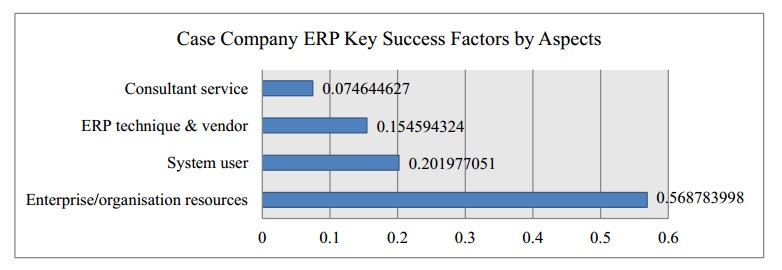
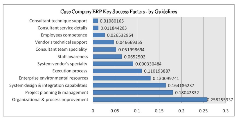
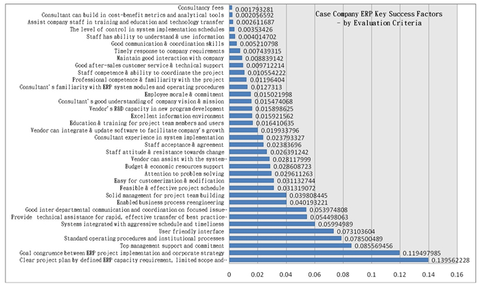
Enterprise resource planning (ERP) systems are software module packages which can be customized up to a certain limit to suit the specific needs of each organization. Many ERP projects have not been effective at achieving all of the intended results due to high cost and high failure risks in ERP implementation. This study integrates the prior theories and knowledge gained from several textile industry practitioners for ERP projects. A two-stage method involving the Delphi and analytic hierarchy process decision support methodology was conducted. Based on the case of the textile industry in Taiwan, the findings illustrate the top 10 key factors: a clear project plan by defined ERP capacity requirement; a limited scope and focused flowchart; goal congruence between ERP project implementation and corporate strategy; top management support and commitment; the extent of standard operating procedures and institutional processes; a user-friendly interface; systems integrated with aggressive schedules and timelines; provision of technical assistance for rapid, effective transfer of best practice interventions; good interdepartmental communication and coordination on a focused issue solution; and enablement of business process reengineering and solid management for project team building. The findings of this research will be beneficial to those apparel companies that adopted the ERP.
Citation: Yueh-Hsia Huang, Lan Sun, Tyng-Bin Ger. An analysis of enterprise resource planning systems and key determinants using the Delphi method and an analytic hierarchy process[J]. Data Science in Finance and Economics, 2023, 3(2): 166-183. doi: 10.3934/DSFE.2023010
Enterprise resource planning (ERP) systems are software module packages which can be customized up to a certain limit to suit the specific needs of each organization. Many ERP projects have not been effective at achieving all of the intended results due to high cost and high failure risks in ERP implementation. This study integrates the prior theories and knowledge gained from several textile industry practitioners for ERP projects. A two-stage method involving the Delphi and analytic hierarchy process decision support methodology was conducted. Based on the case of the textile industry in Taiwan, the findings illustrate the top 10 key factors: a clear project plan by defined ERP capacity requirement; a limited scope and focused flowchart; goal congruence between ERP project implementation and corporate strategy; top management support and commitment; the extent of standard operating procedures and institutional processes; a user-friendly interface; systems integrated with aggressive schedules and timelines; provision of technical assistance for rapid, effective transfer of best practice interventions; good interdepartmental communication and coordination on a focused issue solution; and enablement of business process reengineering and solid management for project team building. The findings of this research will be beneficial to those apparel companies that adopted the ERP.

| [1] | Bai R, Li GG, Zeng WJ, et al. (2007) Discuss the influencing factors of the ERP system implementation from the aspects of organization, science and technology - multiple case studies of Taiwan enterprises. J E-bus 5: 175–196. |
| [2] |
Basoglu N, Daim T, Kerimoglu O (2007) Organizational adoption of enterprise resource planning systems: A conceptual framework. J High Technol Mana Res 18: 73–97. https://doi.org/10.1016/j.hitech.2007.03.005 doi: 10.1016/j.hitech.2007.03.005

|
| [3] |
Beatty RC, Williams CD (2006) ERP Ⅱ: best practices for successfully implementing and ERP upgrade. Commu Acm 49: 105–109. https://doi.org/10.1145/1118178.1118184 doi: 10.1145/1118178.1118184
|
| [4] |
Bradley J (2008) Management based critical success factors in the implementation of enterprise resource planning systems. Int J Accountin Inf Syst 9: 175–200. https://doi.org/10.1016/j.accinf.2008.04.001 doi: 10.1016/j.accinf.2008.04.001
|
| [5] |
Bingi, P, Sharma MK, Godla Jk (1999) Critical issues affecting ERP implementation. Inf Syst Manag 16: 7–14. https://doi.org/10.1201/1078/43197.16.3.19990601/31310.2 doi: 10.1201/1078/43197.16.3.19990601/31310.2
|
| [6] | Cai YY (1999) The key success factors in ERP system implementation in Taiwan electronics industry (Master thesis), National Chung Hsing University, Research Center of Business Administration, Taichung. |
| [7] | Chauhan R, Dwivedi R, Sherry AM (2012) Critical success factors for offshoring of enterprise resource planning (ERP) implementations. Bus Syst Res 3: 4–13. Available from: https://hrcak.srce.hr/ojs/index.php/bsr/article/view/12485. |
| [8] | Dai Qinhe (2007) Discussion on the key success factors in upgrading ERP software - the case of electronics industry (Master thesis), Department of Information Management, Yuanzhong University, Taoyuan. |
| [9] | Daniel DR (1961) Management Information Crisis. Harvard Bus Rev 39: 111–121. Available from: https://cir.nii.ac.jp/crid/1571417125685235712. |
| [10] | Davenport TH (1998) Putting the Enterprise into the Enterprise System. Harvard Business School Press. |
| [11] | Gu Yun (1999) Understanding of ERP. Inf Comput 228: 40–43. |
| [12] | Huang ZH, Lin GH (2012) The use of network analysis to explore the key success factors in enterprise ERP system implementation. J Engi Technol Educ 9: 335–367. |
| [13] | Huang Sien (2006) Applying AHP to explore key success factors of ERP for manufacturing sector (Master thesis). Department of Information Management, Private Kaian University, Taoyuan. |
| [14] |
Holland C, Light B (1999) A critical success factors model for ERP implementation. IEEE Software 16: 30–36. https://doi.org/10.1109/52.765784 doi: 10.1109/52.765784
|
| [15] |
Kim Y, Lee Z, Gosain S (2005) Impediments to successful ERP implementation process. Bus Process Manag J 11: 158–170. https://doi.org/10.1108/14637150510591156 doi: 10.1108/14637150510591156
|
| [16] |
Kwahk KY, Lee JN (2008) The role of readiness for change in ERP implementation: Theoretical bases and empirical validation. Inf Manag 45: 474–481. https://doi.org/10.1016/j.im.2008.07.002 doi: 10.1016/j.im.2008.07.002
|
| [17] | Laughlin SP (1999) An ERP game plan. J Bus Strateg 20: 32–37. |
| [18] | Lin XJ (2010) A study of key success factors of small and medium-sized enterprises in ERP implementation (Master thesis), National Cheng Kung University Master Program in Top Management, Taiwan Tainan. |
| [19] | Liu YT (2003) Research on the key success factors for importing Oracle ERP systems (Master thesis), Information Management Research Center, National Central University, Taoyuan. |
| [20] | Linstone HA (1978) The Delphi technique. In J. Fowlers (Ed.), Handbook of futures research. Westport, CT: Greenwood Press, 273–300 |
| [21] | Martin MH (1998) Smart managing: best practices, careers, and ideas. Fortune 137: 149–51. |
| [22] | Maskell BH (1991) Performance measurement for world class manufacturing: A model for American companies, Productivity Press, NY. |
| [23] |
Morteza M, Zare RA (2013) Developing a practical framework for assessing ERP post-implementation success using fuzzy analytic network process. Int J Prod Res 51: 1236–1257. https://doi.org/10.1080/00207543.2012.698318 doi: 10.1080/00207543.2012.698318
|
| [24] |
Nah FFH (2006) Critical success factors for enterprise resource planning implementation and upgrade. J Comput Inf Syst 46: 99–113. https://doi.org/10.1080/08874417.2006.11645928 doi: 10.1080/08874417.2006.11645928
|
| [25] | Oliver R (1999) ERP is dead, long live ERP. Manag Rev 88: 12–13. |
| [26] |
Olson DL, Zhao F (2007) CIOs' perspectives of critical success factors in ERP upgrade projects. Enterp Inf Syst 1: 129–138. https://doi.org/10.1080/17517570601088364 doi: 10.1080/17517570601088364
|
| [27] |
Olson DL, Chae BK, Sheu C (2013) Relative impact of different ERP forms on global manufacturing organisations: An exploratory analysis of a global manufacturing survey. Int J Prod Res 51: 1520–1534. https://doi.org/10.1080/00207543.2012.701772 doi: 10.1080/00207543.2012.701772
|
| [28] |
Olson DL, Staley J (2012) Case study of open-source enterprise resource planning implementation in a small business. Enter Inf Syst 6: 79–94. https://doi.org/10.1080/17517575.2011.566697 doi: 10.1080/17517575.2011.566697
|
| [29] | Parr A, Shanks G (2000) A model of ERP project implementation. J Inf Technol 15: 289–303. |
| [30] | Ragowsky A, Somers TM (2002) Special section: Enterprise resource planning. J Manag Inf Syst 19: 11–16. |
| [31] | Saaty TL (2000) Fundamentals of decision making and priority theory with the analytic hierarchy process (Analytic Hierarchy Process Series, Vol. 6). Pittsburgh, PA: Rws Publications. |
| [32] | Shanley A (eds.) (1997) ERP in CPI: nine steps to successful implementation. Chemical Engineering, 86–88. Available from: http://www.chemengonline.com/articles/1985-1999/Vol104/chevol104_num11_135.html. |
| [33] | SME Department of the Ministry of Economic Affairs (2010) White Paper on SMEs in the Ministry of Economic Affairs, China Institute of Economic Research. Available from: http://book.moeasmea.gov.tw/book/doc_detail.jsp?pub_SerialNo = 2010A01016 & click = 2010A01016. |
| [34] | SME Department of the Ministry of Economic Affairs (2019) White Paper on SMEs in the Ministry of Economic Affairs, China Institute of Economic Research. Available from: https://www.facebook.com/smea.gov.tw/photos/a.436225466719404/1182200378788572/?type = 3 & theater. |
| [35] | Sumner M (2006) Critical Success Factors in ERP Implementation: Five Years Laster. Proceedings of Americas Conference on Information Systems (AMCIS). 305–316. |
| [36] | Vasilash GS (1997) How to and how not to implement ERP. Automotive Manufacturing & Production, 109: 64–65. |
| [37] | Wall SJ, McKineey RS (1998) Wall-to-wall change. Across The Board, 37: 32–38. |
| [38] | West RN (1998) Up and running in nine months. Manag Account 80: 20–27. |
| [39] | Wu CX, Huang QP (2008) Using Delphi Method to explore the key success factors for SMEs in importing ERP, presented to 2008 Global Operations and Management and Industry Practice Symposium, Taiwan. |
| [40] | Xie FY (2001) The use of balance scorecard in analysing ERP system and performance evaluation system (Master thesis), Department of Accounting, Tamkang University, Taipei. |
| [41] | Xu WK (2000) Exploring the key factors in business ERP implementation (Master thesis), Department of Industrial Management, National Taiwan University of Science and Technology, Taipei. |
| [42] | Ye ML, Chen MY (2005) SMEs and ERP key success factors, the third Management Concept and Practice Symposium Proceedings, 37–61. |
| [43] | Zhang SB (2000) A study of ERP key success factors in the electronics industry (Master thesis), Private Yuan Zhi University Industrial Engineering Research Center, Taiwan Taoyuan. |
| [44] | Zhang TX, Wang XY, Lin HQ (2013) An investigation of second ERP implementation key success factors in small and medium-sized enterprises - the case of S Company in responding to IFRS, 2013 International ERP Academic and Practical Seminar. Available from: http://www.xedu.biz/cerps.org.tw/downloads/2013conf_paper/C3-2.pdf. |
Figures(3) / Tables(6)
Yueh-Hsia Huang, Lan Sun, Tyng-Bin Ger. An analysis of enterprise resource planning systems and key determinants using the Delphi method and an analytic hierarchy process[J]. Data Science in Finance and Economics, 2023, 3(2): 166-183. doi: 10.3934/DSFE.2023010


 DownLoad: