DNase I hypersensitive sites (DHSs) are a specific genomic region, which is critical to detect or understand cis-regulatory elements. Although there are many methods developed to detect DHSs, there is a big gap in practice. We presented a deep learning-based language model for predicting DHSs, named LangMoDHS. The LangMoDHS mainly comprised the convolutional neural network (CNN), the bi-directional long short-term memory (Bi-LSTM) and the feed-forward attention. The CNN and the Bi-LSTM were stacked in a parallel manner, which was helpful to accumulate multiple-view representations from primary DNA sequences. We conducted 5-fold cross-validations and independent tests over 14 tissues and 4 developmental stages. The empirical experiments showed that the LangMoDHS is competitive with or slightly better than the iDHS-Deep, which is the latest method for predicting DHSs. The empirical experiments also implied substantial contribution of the CNN, Bi-LSTM, and attention to DHSs prediction. We implemented the LangMoDHS as a user-friendly web server which is accessible at http:/www.biolscience.cn/LangMoDHS/. We used indices related to information entropy to explore the sequence motif of DHSs. The analysis provided a certain insight into the DHSs.
Citation: Xingyu Tang, Peijie Zheng, Yuewu Liu, Yuhua Yao, Guohua Huang. LangMoDHS: A deep learning language model for predicting DNase I hypersensitive sites in mouse genome[J]. Mathematical Biosciences and Engineering, 2023, 20(1): 1037-1057. doi: 10.3934/mbe.2023048
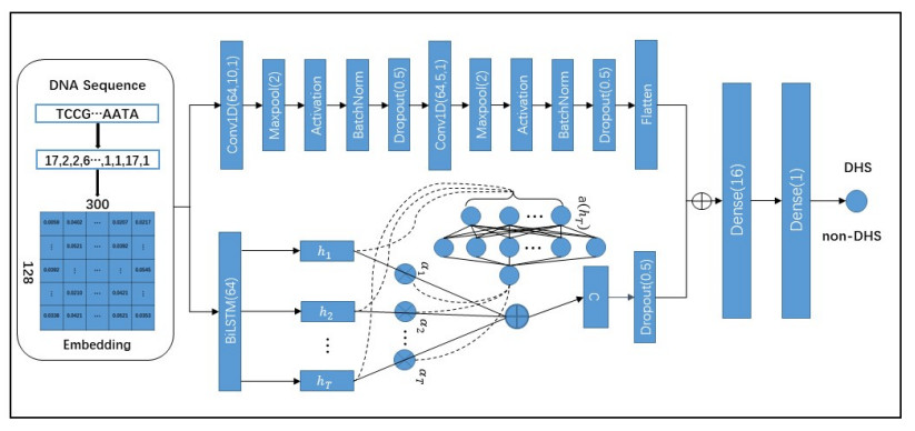
DNase I hypersensitive sites (DHSs) are a specific genomic region, which is critical to detect or understand cis-regulatory elements. Although there are many methods developed to detect DHSs, there is a big gap in practice. We presented a deep learning-based language model for predicting DHSs, named LangMoDHS. The LangMoDHS mainly comprised the convolutional neural network (CNN), the bi-directional long short-term memory (Bi-LSTM) and the feed-forward attention. The CNN and the Bi-LSTM were stacked in a parallel manner, which was helpful to accumulate multiple-view representations from primary DNA sequences. We conducted 5-fold cross-validations and independent tests over 14 tissues and 4 developmental stages. The empirical experiments showed that the LangMoDHS is competitive with or slightly better than the iDHS-Deep, which is the latest method for predicting DHSs. The empirical experiments also implied substantial contribution of the CNN, Bi-LSTM, and attention to DHSs prediction. We implemented the LangMoDHS as a user-friendly web server which is accessible at http:/www.biolscience.cn/LangMoDHS/. We used indices related to information entropy to explore the sequence motif of DHSs. The analysis provided a certain insight into the DHSs.

| [1] |
T. Zhang, A. P. Marand, J. Jiang, PlantDHS: A database for DNase I hypersensitive sites in plants, Nucleic. Acids. Res., 44 (2016), D1148–D1153. https://doi.org/10.1093/nar/gkv962 doi: 10.1093/nar/gkv962

|
| [2] |
D. S. Gross, W. T. Garrard, Nuclease hypersensitive sites in chromatin, Annu. Rev. Biochem., 57 (1988), 159–197. https://doi.org/10.1146/annurev.bi.57.070188.001111 doi: 10.1146/annurev.bi.57.070188.001111
|
| [3] |
G. E. Crawford, I. E. Holt, J. C. Mullikin, D. Tai, E. D. Green, T. G. Wolfsberg, et al., Identifying gene regulatory elements by genome-wide recovery of DNase hypersensitive sites, Proc. Natl. Acad. Sci., 101 (2004), 992–997. https://doi.org/10.1073/pnas.0307540100 doi: 10.1073/pnas.0307540100
|
| [4] |
M. M. Carrasquillo, M. Allen, J. D. Burgess, X. Wang, S. L. Strickland, S. Aryal, et al., A candidate regulatory variant at the TREM gene cluster associates with decreased Alzheimer's disease risk and increased TREML1 and TREM2 brain gene expression, Alzheimer's Dementia, 13 (2017), 663–673. https://doi.org/10.1016/j.jalz.2016.10.005 doi: 10.1016/j.jalz.2016.10.005
|
| [5] |
W. Meuleman, A. Muratov, E. Rynes, J. Halow, K. Lee, D. Bates, et al., Index and biological spectrum of human DNase I hypersensitive sites, Nature, 584 (2020), 244–251. https://doi.org/10.1038/s41586-020-2559-3 doi: 10.1038/s41586-020-2559-3
|
| [6] |
M. T. Maurano, R. Humbert, E. Rynes, R. E. Thurman, E. Haugen, H. Wang, et al., Systematic localization of common disease-associated variation in regulatory DNA, Science, 337 (2012), 1190–1195. https://doi.org/10.1126/science.1222794 doi: 10.1126/science.1222794
|
| [7] |
J. Ernst, P. Kheradpour, T. S. Mikkelsen, N. Shoresh, L. D. Ward, C. B. Epstein, et al., Mapping and analysis of chromatin state dynamics in nine human cell types, Nature, 473 (2011), 43–49. https://doi.org/10.1038/nature09906 doi: 10.1038/nature09906
|
| [8] |
M. Mokry, M. Harakalova, F. W. Asselbergs, P. I. de Bakker, E. E. Nieuwenhuis, Extensive association of common disease variants with regulatory sequence, PLoS One, 11 (2016), e0165893. https://doi.org/10.1371/journal.pone.0165893 doi: 10.1371/journal.pone.0165893
|
| [9] |
D. Weghorn, F. Coulet, K. M. Olson, C. DeBoever, F. Drees, A. Arias, et al., Identifying DNase I hypersensitive sites as driver distal regulatory elements in breast cancer, Nat. Commun., 8 (2017), 1–16. https://doi.org/10.1038/s41467-017-00100-x doi: 10.1038/s41467-017-00100-x
|
| [10] |
W. Jin, Q. Tang, M. Wan, K. Cui, Y. Zhang, G. Ren, et al., Genome-wide detection of DNase I hypersensitive sites in single cells and FFPE tissue samples, Nature, 528 (2015), 142–146. https://doi.org/10.1038/nature15740 doi: 10.1038/nature15740
|
| [11] |
G. E. Crawford, S. Davis, P. C. Scacheri, G. Renaud, M. J. Halawi, M. R. Erdos, et al., DNase-chip: A high-resolution method to identify DNase I hypersensitive sites using tiled microarrays, Nat. Methods, 3 (2006), 503–509. https://doi.org/10.1038/nmeth888 doi: 10.1038/nmeth888
|
| [12] |
J. Cooper, Y. Ding, J. Song, K. Zhao, Genome-wide mapping of DNase I hypersensitive sites in rare cell populations using single-cell DNase sequencing, Nat. Protoc., 12 (2017), 2342–2354. https://doi.org/10.1038/nprot.2017.099 doi: 10.1038/nprot.2017.099
|
| [13] |
G. E. Crawford, I. E. Holt, J. Whittle, B. D. Webb, D. Tai, S. Davis, et al., Genome-wide mapping of DNase hypersensitive sites using massively parallel signature sequencing (MPSS), Genome Res., 16 (2006), 123–131. https://doi.org/10.1101/gr.4074106 doi: 10.1101/gr.4074106
|
| [14] |
L. Song, G. E. Crawford, DNase-seq: A high-resolution technique for mapping active gene regulatory elements across the genome from mammalian cells, Cold Spring Harbor Protoc., 2010 (2010), pdb.prot5384. https://doi.org/10.1101/pdb.prot5384 doi: 10.1101/pdb.prot5384
|
| [15] | W. Zhang, J. Jiang, Genome-wide mapping of DNase I hypersensitive sites in plants, in Plant Functional Genomics, Humana Press, 1284 (2015), 71–89. https://doi.org/10.1007/978-1-4939-2444-8_4 |
| [16] |
Y. Wang, K. Wang, Genome-wide identification of DNase I hypersensitive sites in plants, Curr. Protoc., 1 (2021), e148. https://doi.org/10.1002/cpz1.148 doi: 10.1002/cpz1.148
|
| [17] |
S. Wang, Q. Zhang, Z. Shen, Y. He, Z. Chen, J. Li, et al., Predicting transcription factor binding sites using DNA shape features based on shared hybrid deep learning architecture, Mol. Ther. Nucleic Acids, 24 (2021), 154–163. https://doi.org/10.1016/j.omtn.2021.02.014 doi: 10.1016/j.omtn.2021.02.014
|
| [18] |
Q. Zhang, Y. He, S. Wang, Z. Chen, Z. Guo, Z. Cui, et al., Base-resolution prediction of transcription factor binding signals by a deep learning framework, PLoS Comp. Biol., 18 (2022), e1009941. https://doi.org/10.1371/journal.pcbi.1009941 doi: 10.1371/journal.pcbi.1009941
|
| [19] |
S. Wang, Y. He, Z. Chen, Q. Zhang, FCNGRU: Locating transcription factor binding sites by combing fully convolutional neural network with gated recurrent unit, IEEE J. Biomed. Health. Inf., 26 (2021), 1883–1890. https://doi.org/10.1109/JBHI.2021.3117616 doi: 10.1109/JBHI.2021.3117616
|
| [20] |
Q. Zhang, Z. Shen, D. S. Huang, Predicting in-vitro transcription factor binding sites using DNA sequence+ shape, IEEE/ACM Trans. Comput. Biol. Bioinf., 18 (2019), 667–676. https://doi.org/10.1109/TCBB.2019.2947461 doi: 10.1109/TCBB.2019.2947461
|
| [21] |
Q. Zhang, S. Wang, Z. Chen, Y. He, Q. Liu, D. S. Huang, Locating transcription factor binding sites by fully convolutional neural network, Briefings Bioinf., 22 (2021), bbaa435. https://doi.org/10.1093/bib/bbaa435 doi: 10.1093/bib/bbaa435
|
| [22] |
Y. Zhang, Z. Wang, Y. Zeng, Y. Liu, S. Xiong, M. Wang, et al., A novel convolution attention model for predicting transcription factor binding sites by combination of sequence and shape, Briefings Bioinf., 23 (2022), bbab525. https://doi.org/10.1093/bib/bbab525 doi: 10.1093/bib/bbab525
|
| [23] |
Y. Zhang, Z. Wang, Y. Zeng, J. Zhou, Q. Zou, High-resolution transcription factor binding sites prediction improved performance and interpretability by deep learning method, Briefings Bioinf., 22 (2021), bbab273. https://doi.org/10.1093/bib/bbab273 doi: 10.1093/bib/bbab273
|
| [24] |
Y. He, Z. Shen, Q. Zhang, S. Wang, D. S. Huang, A survey on deep learning in DNA/RNA motif mining, Briefings Bioinf., 22 (2021), bbaa229. https://doi.org/10.1093/bib/bbaa229 doi: 10.1093/bib/bbaa229
|
| [25] |
W. S. Noble, S. Kuehn, R. Thurman, M. Yu, J. Stamatoyannopoulos, Predicting the in vivo signature of human gene regulatory sequences, Bioinformatics, 21 (2005), i338–i343. https://doi.org/10.1093/bioinformatics/bti1047 doi: 10.1093/bioinformatics/bti1047
|
| [26] |
B. Manavalan, T. H. Shin, G. Lee, DHSpred: Support-vector-machine-based human DNase I hypersensitive sites prediction using the optimal features selected by random forest, Oncotarget, 9 (2018), 1944. https://doi.org/10.18632/oncotarget.23099 doi: 10.18632/oncotarget.23099
|
| [27] |
S. Zhang, W. Zhuang, Z. Xu, Prediction of DNase I hypersensitive sites in plant genome using multiple modes of pseudo components, Anal. Biochem., 549 (2018), 149–156. https://doi.org/10.1016/j.ab.2018.03.025 doi: 10.1016/j.ab.2018.03.025
|
| [28] |
Y. Liang, S. Zhang, IDHS-DMCAC: Identifying DNase I hypersensitive sites with balanced dinucleotide-based detrending moving-average cross-correlation coefficient, SAR QSAR Environ. Res., 30 (2019), 429–445. https://doi.org/10.1080/1062936X.2019.1615546 doi: 10.1080/1062936X.2019.1615546
|
| [29] |
S. Zhang, Z. Duan, W. Yang, C. Qian, Y. You, IDHS-DASTS: Identifying DNase I hypersensitive sites based on LASSO and stacking learning, Mol. Omics, 17 (2021), 130–141. https://doi.org/10.1039/D0MO00115E doi: 10.1039/D0MO00115E
|
| [30] |
B. Liu, R. Long, K. C. Chou, IDHS-EL: Identifying DNase I hypersensitive sites by fusing three different modes of pseudo nucleotide composition into an ensemble learning framework, Bioinformatics, 32 (2016), 2411–2418. https://doi.org/10.1093/bioinformatics/btw186 doi: 10.1093/bioinformatics/btw186
|
| [31] |
S. Zhang, J. Lin, L. Su, Z. Zhou, PDHS-DSET: Prediction of DNase I hypersensitive sites in plant genome using DS evidence theory, Anal. Biochem., 564 (2019), 54–63. https://doi.org/10.1016/j.ab.2018.10.018 doi: 10.1016/j.ab.2018.10.018
|
| [32] |
Y. Zheng, H. Wang, Y. Ding, F. Guo, CEPZ: A novel predictor for identification of DNase I hypersensitive sites, IEEE/ACM Trans. Comput. Biol. Bioinf., 18 (2021), 2768–2774. https://doi.org/10.1109/TCBB.2021.3053661 doi: 10.1109/TCBB.2021.3053661
|
| [33] |
S. Zhang, Q. Yu, H. He, F. Zhu, P. Wu, L. Gu, et al., IDHS-DSAMS: Identifying DNase I hypersensitive sites based on the dinucleotide property matrix and ensemble bagged tree, Genomics, 112 (2020), 1282–1289. https://doi.org/10.1016/j.ygeno.2019.07.017 doi: 10.1016/j.ygeno.2019.07.017
|
| [34] |
S. Zhang, T. Xue, Use Chou's 5-steps rule to identify DNase I hypersensitive sites via dinucleotide property matrix and extreme gradient boosting, Mol. Genet. Genomics, 295 (2020), 1431–1442. https://doi.org/10.1007/s00438-020-01711-8 doi: 10.1007/s00438-020-01711-8
|
| [35] |
Z. C. Xu, S. Y. Jiang, W. R. Qiu, Y. C. Liu, X. Xiao, IDHSs-PseTNC: Identifying DNase I hypersensitive sites with pseuo trinucleotide component by deep sparse auto-encoder, Lett. Org. Chem., 14 (2017), 655–664. https://doi.org/10.2174/1570178614666170213102455 doi: 10.2174/1570178614666170213102455
|
| [36] |
C. Lyu, L. Wang, J. Zhang, Deep learning for DNase I hypersensitive sites identification, BMC genomics, 19 (2018), 155–165. https://doi.org/10.1186/s12864-018-5283-8 doi: 10.1186/s12864-018-5283-8
|
| [37] |
P. Feng, N. Jiang, N. Liu, Prediction of DNase I hypersensitive sites by using pseudo nucleotide compositions, Sci. World J., 2014 (2014), 740506. https://doi.org/10.1155/2014/740506 doi: 10.1155/2014/740506
|
| [38] |
W. Chen, T. Y. Lei, D. C. Jin, H. Lin, K. C. Chou, PseKNC: A flexible web server for generating pseudo K-tuple nucleotide composition, Anal. Biochem., 456 (2014), 53–60. https://doi.org/10.1016/j.ab.2014.04.001 doi: 10.1016/j.ab.2014.04.001
|
| [39] |
W. Chen, H. Lin, K. C. Chou, Pseudo nucleotide composition or PseKNC: An effective formulation for analyzing genomic sequences, Mol. Biosyst., 11 (2015), 2620–2634. https://doi.org/10.1039/C5MB00155B doi: 10.1039/C5MB00155B
|
| [40] |
B. Liu, F. Liu, X. Wang, J. Chen, L. Fang, K. C. Chou, Pse-in-One: A web server for generating various modes of pseudo components of DNA, RNA, and protein sequences, Nucleic Acids Res., 43 (2015), W65–W71. https://doi.org/10.1093/nar/gkv458 doi: 10.1093/nar/gkv458
|
| [41] |
S. Zhang, Z. Zhou, X. Chen, Y. Hu, L. Yang, PDHS-SVM: A prediction method for plant DNase I hypersensitive sites based on support vector machine, J. Theor. Biol., 426 (2017), 126–133. https://doi.org/10.1016/j.jtbi.2017.05.030 doi: 10.1016/j.jtbi.2017.05.030
|
| [42] |
K. He, X. Zhang, S. Ren, J. Sun, Spatial pyramid pooling in deep convolutional networks for visual recognition, IEEE Trans. Pattern Anal. Mach. Intell., 37 (2015), 1904–1916. https://doi.org/10.1109/TPAMI.2015.2389824 doi: 10.1109/TPAMI.2015.2389824
|
| [43] |
F. Y. Dao, H. Lv, W. Su, Z. J. Sun, Q. L. Huang, H. Lin, IDHS-deep: an integrated tool for predicting DNase I hypersensitive sites by deep neural network, Briefings Bioinf., 22 (2021), bbab047. https://doi.org/10.1093/bib/bbab047 doi: 10.1093/bib/bbab047
|
| [44] |
C. E. Breeze, J. Lazar, T. Mercer, J. Halow, I. Washington, K. Lee, et al., Atlas and developmental dynamics of mouse DNase I hypersensitive sites, bioRxiv, 2020 (2020). https://doi.org/10.1101/2020.06.26.172718 doi: 10.1101/2020.06.26.172718
|
| [45] |
W. Li, A. Godzik, Cd-hit: A fast program for clustering and comparing large sets of protein or nucleotide sequences, Bioinformatics, 22 (2006), 1658–1659. https://doi.org/10.1093/bioinformatics/btl158 doi: 10.1093/bioinformatics/btl158
|
| [46] |
L. Fu, B. Niu, Z. Zhu, S. Wu, W. Li, CD-HIT: Accelerated for clustering the next-generation sequencing data, Bioinformatics, 28 (2012), 3150–3152. https://doi.org/10.1093/bioinformatics/bts565 doi: 10.1093/bioinformatics/bts565
|
| [47] |
X. Tang, P. Zheng, X. Li, H. Wu, D. Q. Wei, Y. Liu, et al., Deep6mAPred: A CNN and Bi-LSTM-based deep learning method for predicting DNA N6-methyladenosine sites across plant species, Methods, 204 (2022), 142–150. https://doi.org/10.1016/j.ymeth.2022.04.011 doi: 10.1016/j.ymeth.2022.04.011
|
| [48] | T. Mikolov, K. Chen, G. Corrado, J. Dean, Efficient estimation of word representations in vector space, preprint, arXiv: 1301.3781. |
| [49] | T. Mikolov, I. Sutskever, K. Chen, G. S. Corrado, J. Dean, Distributed representations of words and phrases and their compositionality, in Advances in neural information processing systems, 26 (2013), 3111–3119. |
| [50] |
K. Fukushima, S. Miyake, Neocognitron: A new algorithm for pattern recognition tolerant of deformations and shifts in position, Pattern Recognt., 15 (1982), 455–469. https://doi.org/10.1016/0031-3203(82)90024-3 doi: 10.1016/0031-3203(82)90024-3
|
| [51] |
D. H. Hubel, T. N. Wiesel, Receptive fields, binocular interaction and functional architecture in the cat's visual cortex, J. Physiol., 160 (1962), 106. https://doi.org/10.1113/jphysiol.1962.sp006837 doi: 10.1113/jphysiol.1962.sp006837
|
| [52] | Y. LeCun, B. Boser, J. Denker, D. Henderson, R. Howard, W. Hubbard, et al., Handwritten digit recognition with a back-propagation network, in Advances in neural information processing systems, Morgan Kaufmann, 2 (1989), 396–404. |
| [53] |
S. Hochreiter, J. Schmidhuber, Long short-term memory, Neural Comput., 9 (1997), 1735–1780. https://doi.org/10.1162/neco.1997.9.8.1735 doi: 10.1162/neco.1997.9.8.1735
|
| [54] | A. Vaswani, N. Shazeer, N. Parmar, J. Uszkoreit, L. Jones, A. N. Gomez, et al., Attention is all you need, in Advances in neural information processing systems, 30 (2017), 6000–6010. |
| [55] | C. Raffel, D. P. Ellis, Feed-forward networks with attention can solve some long-term memory problems, preprint, arXiv: 1512.08756. |


Figures(9) / Tables(6)

Xingyu Tang, Peijie Zheng, Yuewu Liu, Yuhua Yao, Guohua Huang. LangMoDHS: A deep learning language model for predicting DNase I hypersensitive sites in mouse genome[J]. Mathematical Biosciences and Engineering, 2023, 20(1): 1037-1057. doi: 10.3934/mbe.2023048


 DownLoad: