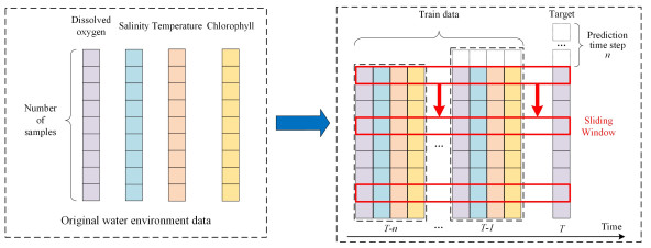
As an essential water quality parameter in aquaculture ponds, dissolved oxygen (DO) affects the growth and development of aquatic animals and their feeding and absorption. However, DO is easily influenced by external factors. It is not easy to make scientific and accurate predictions of DO concentration trends, especially in long-term predictions. This paper uses a one-dimensional convolutional neural network to extract the features of multidimensional input data. Bidirectional long and short-term memory neural network propagated forward and backward twice and thoroughly mined the before and after attribute relationship of each data of dissolved oxygen sequence. The attention mechanism focuses the model on the time series prediction step to improve long-term prediction accuracy. Finally, we built an integrated prediction model based on convolutional neural network (CNN), bidirectional long and short-term memory neural network (BiLSTM) and attention mechanism (AM), which is called CNN-BiLSTM-AM model. To determine the accuracy of the CNN-BiLSTM-AM model, we conducted short-term (30 minutes, one hour) and long-term (6 hours, 12 hours) experimental validation on real datasets monitored at two aquaculture farms in Yantai City, Shandong Province, China. Meanwhile, the performance was compared and visualized with support vector regression, recurrent neural network, long short-term memory neural network, CNN-LSTM model and CNN-BiLSTM model. The results show that compared with other comparative models, the proposed CNN-BiLSTM-AM model has an excellent performance in mean absolute error, root means square error, mean absolute percentage error and determination coefficient.
Citation: Wenbo Yang, Wei Liu, Qun Gao. Prediction of dissolved oxygen concentration in aquaculture based on attention mechanism and combined neural network[J]. Mathematical Biosciences and Engineering, 2023, 20(1): 998-1017. doi: 10.3934/mbe.2023046
As an essential water quality parameter in aquaculture ponds, dissolved oxygen (DO) affects the growth and development of aquatic animals and their feeding and absorption. However, DO is easily influenced by external factors. It is not easy to make scientific and accurate predictions of DO concentration trends, especially in long-term predictions. This paper uses a one-dimensional convolutional neural network to extract the features of multidimensional input data. Bidirectional long and short-term memory neural network propagated forward and backward twice and thoroughly mined the before and after attribute relationship of each data of dissolved oxygen sequence. The attention mechanism focuses the model on the time series prediction step to improve long-term prediction accuracy. Finally, we built an integrated prediction model based on convolutional neural network (CNN), bidirectional long and short-term memory neural network (BiLSTM) and attention mechanism (AM), which is called CNN-BiLSTM-AM model. To determine the accuracy of the CNN-BiLSTM-AM model, we conducted short-term (30 minutes, one hour) and long-term (6 hours, 12 hours) experimental validation on real datasets monitored at two aquaculture farms in Yantai City, Shandong Province, China. Meanwhile, the performance was compared and visualized with support vector regression, recurrent neural network, long short-term memory neural network, CNN-LSTM model and CNN-BiLSTM model. The results show that compared with other comparative models, the proposed CNN-BiLSTM-AM model has an excellent performance in mean absolute error, root means square error, mean absolute percentage error and determination coefficient.

| [1] | Agriculture Organization of the United Nations, Fisheries Department, The State of World Fisheries and Aquaculture, Food & Agriculture Org, 2000. |
| [2] |
X. Li, J. Li, Y. Wang, L. Fu, Y. Fu, B. Li, et al., Aquaculture industry in china: Current state, challenges, and outlook, Rev. Fish. Sci., 19 (2011), 187–200. https://doi.org/10.1080/10641262.2011.573597 doi: 10.1080/10641262.2011.573597

|
| [3] |
J. Huan, H. Li, M. Li, B. Chen, Prediction of dissolved oxygen in aquaculture based on gradient boosting decision tree and long short-term memory network: A study of Chang Zhou fishery demonstration base, China, Comput. Electron. Agric., 175 (2020), 105530. https://doi.org/10.1016/j.compag.2020.105530 doi: 10.1016/j.compag.2020.105530
|
| [4] |
S. Midilli, D. Çoban, M. Güler, S. Küçük, Gas bubble disease in nile tilapia and hybrid red tilapia (cichlidae, oreochromis spp.) under culture conditions, J. Fish. Aquat. Sci., 36 (2019), 285–291. http://dx.doi.org/10.12714/egejfas.2019.36.3.09 doi: 10.12714/egejfas.2019.36.3.09
|
| [5] |
C. E. Boyd, E. L. Torrans, C. S. Tucker, Dissolved oxygen and aeration in ictalurid catfish aquaculture, J. World Aquacult. Soc., 49 (2018), 7–70. https://doi.org/10.1111/jwas.12469 doi: 10.1111/jwas.12469
|
| [6] |
A. Sentas, L. Karamoutsou, N. Charizopoulos, T. Psilovikos, A. Psilovikos, A. Loukas, The use of stochastic models for short-term prediction of water parameters of the thesaurus dam, River Nestos, Greece, Proceedings, 2 (2018), 634. https://doi.org/10.3390/proceedings2110634 doi: 10.3390/proceedings2110634
|
| [7] |
M. Valera, R. K. Walter, B. A. Bailey, J. E. Castillo, Machine learning based predictions of dissolved oxygen in a small coastal embayment, J. Mar. Sci. Eng., 8 (2020), 1007. https://doi.org/10.3390/jmse8121007 doi: 10.3390/jmse8121007
|
| [8] |
C. Xu, X. Chen, L. Zhang, Predicting river dissolved oxygen time series based on stand-alone models and hybrid wavelet-based models, J. Environ. Manage., 295 (2021), 113085. https://doi.org/10.1016/j.jenvman.2021.113085 doi: 10.1016/j.jenvman.2021.113085
|
| [9] |
A. Sorjamaa, J. Hao, N. Reyhani, Y. Ji, A. Lendasse, Methodology for long-term prediction of time series, Neurocomputing, 70 (2007), 2861–2869. https://doi.org/10.1016/j.neucom.2006.06.015 doi: 10.1016/j.neucom.2006.06.015
|
| [10] |
M. Längkvist, L. Karlsson, A. Loutfi, A review of unsupervised feature learning and deep learning for time-series modeling, Pattern Recognit. Lett., 42 (2014), 11–24. https://doi.org/10.1016/j.patrec.2014.01.008 doi: 10.1016/j.patrec.2014.01.008
|
| [11] |
L. Karamoutsou, A. Psilovikos, Deep learning in water resources management: The case study of Kastoria lake in Greece, Water, 13 (2021), 3364. https://doi.org/10.3390/w13233364 doi: 10.3390/w13233364
|
| [12] | Q. Ye, X. Yang, C. Chen, J. Wang, River water quality parameters prediction method based on LSTM-RNN model, in 2019 Chinese Control And Decision Conference (CCDC), (2019), 3024–3028. https://doi.org/10.1109/CCDC.2019.8832885 |
| [13] |
J. Yan, Y. Gao, Y. Yu, H. Xu, Z. Xu, A prediction model based on deep belief network and least squares svr applied to cross-section water quality, Water, 12 (2020), 1929. https://doi.org/10.3390/w12071929 doi: 10.3390/w12071929
|
| [14] |
L. Sheng, J. Zhou, X. Li, Y. Pan, L. Liu, Water quality prediction method based on preferred classification, IET Cyber-Phys. Syst. Theory Appl., 5 (2020), 176–180. https://doi.org/10.1049/iet-cps.2019.0062 doi: 10.1049/iet-cps.2019.0062
|
| [15] |
J. Wu, Z. Wang, A hybrid model for water quality prediction based on an artificial neural network, wavelet transform, and long short-term memory, Water, 14 (2022), 610. https://doi.org/10.3390/w14040610 doi: 10.3390/w14040610
|
| [16] |
B. Lim, S. Zohren, Time-series forecasting with deep learning: A survey, Philos. Trans. A Math. Phys. Eng. Sci., 379 (2021), 20200209. https://doi.org/10.1098/rsta.2020.0209 doi: 10.1098/rsta.2020.0209
|
| [17] |
H. Ismail Fawaz, G. Forestier, J. Weber, L. Idoumghar, P. A. Muller, Deep learning for time series classification: A review, Data Min. Knowl. Discovery, 33 (2019), 917–963. https://doi.org/10.1007/s10618-019-00619-1 doi: 10.1007/s10618-019-00619-1
|
| [18] |
P. Shi, G. Li, Y. Yuan, G. Huang, L. Kuang, Prediction of dissolved oxygen content in aquaculture using clustering-based softplus extreme learning machine, Comput. Electron. Agric., 157 (2019), 329–338. https://doi.org/10.1016/j.compag.2019.01.004 doi: 10.1016/j.compag.2019.01.004
|
| [19] |
W. Li, H. Wu, N. Zhu, Y. Jiang, J. Tan, Y. Guo, Prediction of dissolved oxygen in a fishery pond based on gated recurrent unit (GRU), Inf. Process. Agric., 8 (2021), 185–193. https://doi.org/10.1016/j.inpa.2020.02.002 doi: 10.1016/j.inpa.2020.02.002
|
| [20] |
C. Li, Z. Li, J. Wu, L. Zhu, J. Yue, A hybrid model for dissolved oxygen prediction in aquaculture based on multi-scale features, Inf. Process. Agric., 5 (2018), 11–20. https://doi.org/10.1016/j.inpa.2017.11.002 doi: 10.1016/j.inpa.2017.11.002
|
| [21] | Q. Ren, X. Wang, W. Li, Y. Wei, D. An, Research of dissolved oxygen prediction in recirculating aquaculture systems based on deep belief network, Aquacult. Eng., 90 (2020), 102085. |
| [22] |
J. Huang, S. Liu, S. G. Hassan, L. Xu, C. Huang, A hybrid model for short-term dissolved oxygen content prediction, Comput. Electron. Agric., 186 (2021), 106216. https://doi.org/10.1016/j.compag.2021.106216 doi: 10.1016/j.compag.2021.106216
|
| [23] |
H. Liu, R. Yang, Z. Duan, Wind speed forecasting using a new multi-factor fusion and multi-resolution ensemble model with real-time decomposition and adaptive error correction, Energy Convers. Manage., 217 (2020), 112995. https://doi.org/10.1016/j.enconman.2020.112995 doi: 10.1016/j.enconman.2020.112995
|
| [24] | J. Bi, Y. Lin, Q. Dong, H. Yuan, M. Zhou, An improved attention-based lstm for multi-step dissolved oxygen prediction in water environment, in 2020 IEEE International Conference on Networking, Sensing and Control (ICNSC), (2020), 1–6. https://doi.org/10.1109/ICNSC48988.2020.9238097 |
| [25] |
Y. Liu, Q. Zhang, L. Song, Y. Chen, Attention-based recurrent neural networks for accurate short-term and long-term dissolved oxygen prediction, Comput. Electron. Agric., 165 (2019), 104964. https://doi.org/10.1016/j.compag.2019.104964 doi: 10.1016/j.compag.2019.104964
|
| [26] |
X. Yang, B. Liu, Uncertain time series analysis with imprecise observations, Fuzzy Optim. Decis. Making, 18 (2018), 263–278. https://doi.org/10.1007/s10700-018-9298-z doi: 10.1007/s10700-018-9298-z
|
| [27] |
T. Wang, M. Wang, Communication network time series prediction algorithm based on big data method, Wireless Pers. Commun., 102 (2017), 1041–1056. https://doi.org/10.1007/s11277-017-5138-7 doi: 10.1007/s11277-017-5138-7
|
| [28] |
Y. LeCun, B. Boser, J. S. Denker, D. Henderson, R. E. Howard, W. Hubbard, et al., Backpropagation applied to handwritten zip code recognition, Neural Comput., 1 (1989), 541–551. https://doi.org/10.1162/neco.1989.1.4.541 doi: 10.1162/neco.1989.1.4.541
|
| [29] | Á. Zarándy, C. Rekeczky, P. Szolgay, L. O. Chua, Overview of cnn research: 25 years history and the current trends, in 2015 IEEE International Symposium on Circuits and Systems (ISCAS), (2015), 401–404. https://doi.org/10.1109/ISCAS.2015.7168655 |
| [30] |
L. Alzubaidi, J. Zhang, A. J. Humaidi, A. Al-Dujaili, Y. Duan, O. Al-Shamma, et al., Review of deep learning: concepts, cnn architectures, challenges, applications, future directions, J. Big Data, 8 (2021), 53. https://doi.org/10.1186/s40537-021-00444-8 doi: 10.1186/s40537-021-00444-8
|
| [31] | M. Sahu, R. Dash, A survey on deep learning: convolution neural network (CNN), in Intelligent and Cloud Computing, Springer, (2021), 317–325. |
| [32] |
G. Ortac, G. Ozcan, Comparative study of hyperspectral image classification by multidimensional convolutional neural network approaches to improve accuracy, Expert Syst. Appl., 182 (2021), 115280. https://doi.org/10.1016/j.eswa.2021.115280 doi: 10.1016/j.eswa.2021.115280
|
| [33] |
X. Song, Y. Liu, L. Xue, J. Wang, J. Zhang, J. Wang, et al., Time-series well performance prediction based on long short-term memory (LSTM) neural network model, J. Pet. Sci. Eng., 186 (2020), 106682. https://doi.org/10.1016/j.petrol.2019.106682 doi: 10.1016/j.petrol.2019.106682
|
| [34] |
S. Hochreiter, J. Schmidhuber, Long short-term memory, Neural Comput., 9 (1997), 1735–1780. https://doi.org/10.1162/neco.1997.9.8.1735 doi: 10.1162/neco.1997.9.8.1735
|
| [35] |
R. Yu, J. Gao, M. Yu, W. Lu, T. Xu, M. Zhao, et al., LSTM-EFG for wind power forecasting based on sequential correlation features, Future Gener. Comput. Syst., 93 (2019), 33–42. https://doi.org/10.1016/j.future.2018.09.054 doi: 10.1016/j.future.2018.09.054
|
| [36] |
X. Wu, J. Li, Y. Jin, S. Zheng, Modeling and analysis of tool wear prediction based on SVD and BiLSTM, Int. J. Adv. Manuf. Technol., 106 (2020), 4391–4399. https://doi.org/10.1007/s00170-019-04916-3 doi: 10.1007/s00170-019-04916-3
|
| [37] |
M. Schuster, K. K. Paliwal, Bidirectional recurrent neural networks, IEEE Trans. Signal Process., 45 (1997), 2673–2681. https://doi.org/10.1109/78.650093 doi: 10.1109/78.650093
|
| [38] | S. Siami-Namini, N. Tavakoli, A. S. Namin, The performance of LSTM and BiLSTM in forecasting time series, in 2019 IEEE International Conference on Big Data (Big Data), (2019), 3285–3292. https://doi.org/10.1109/BigData47090.2019.9005997 |
| [39] |
Z. Niu, G. Zhong, H. Yu, A review on the attention mechanism of deep learning, Neurocomputing, 452 (2021), 48–62. https://doi.org/10.1016/j.neucom.2021.03.091 doi: 10.1016/j.neucom.2021.03.091
|
| [40] |
A. De Santana Correia, E. L. Colombini, Attention, please! A survey of neural attention models in deep learning, Artif. Intell. Rev., 2022 (2022), 1–88. https://doi.org/10.1007/s10462-022-10148-x doi: 10.1007/s10462-022-10148-x
|


Figures(9) / Tables(6)

Wenbo Yang, Wei Liu, Qun Gao. Prediction of dissolved oxygen concentration in aquaculture based on attention mechanism and combined neural network[J]. Mathematical Biosciences and Engineering, 2023, 20(1): 998-1017. doi: 10.3934/mbe.2023046


 DownLoad: