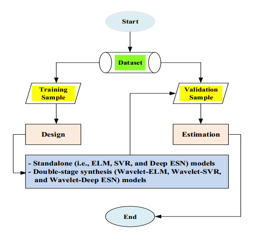
As an indicator measured by incubating organic material from water samples in rivers, the most typical characteristic of water quality items is biochemical oxygen demand (BOD5) concentration, which is a stream pollutant with an extreme circumstance of organic loading and controlling aquatic behavior in the eco-environment. Leading monitoring approaches including machine leaning and deep learning have been evolved for a correct, trustworthy, and low-cost prediction of BOD5 concentration. The addressed research investigated the efficiency of three standalone models including machine learning (extreme learning machine (ELM) and support vector regression (SVR)) and deep learning (deep echo state network (Deep ESN)). In addition, the novel double-stage synthesis models (wavelet-extreme learning machine (Wavelet-ELM), wavelet-support vector regression (Wavelet-SVR), and wavelet-deep echo state network (Wavelet-Deep ESN)) were developed by integrating wavelet transformation (WT) with the different standalone models. Five input associations were supplied for evaluating standalone and double-stage synthesis models by determining diverse water quantity and quality items. The proposed models were assessed using the coefficient of determination (R2), Nash-Sutcliffe (NS) efficiency, and root mean square error (RMSE). The significance of addressed research can be found from the overall outcomes that the predictive accuracy of double-stage synthesis models were not always superior to that of standalone models. Overall results showed that the SVR with 3th distribution (NS = 0.915) and the Wavelet-SVR with 4th distribution (NS = 0.915) demonstrated more correct outcomes for predicting BOD5 concentration compared to alternative models at Hwangji station, and the Wavelet-SVR with 4th distribution (NS = 0.917) was judged to be the most superior model at Toilchun station. In most cases for predicting BOD5 concentration, the novel double-stage synthesis models can be utilized for efficient and organized data administration and regulation of water pollutants on both stations, South Korea.
Citation: Sungwon Kim, Meysam Alizamir, Youngmin Seo, Salim Heddam, Il-Moon Chung, Young-Oh Kim, Ozgur Kisi, Vijay P. Singh. Estimating the incubated river water quality indicator based on machine learning and deep learning paradigms: BOD5 Prediction[J]. Mathematical Biosciences and Engineering, 2022, 19(12): 12744-12773. doi: 10.3934/mbe.2022595
As an indicator measured by incubating organic material from water samples in rivers, the most typical characteristic of water quality items is biochemical oxygen demand (BOD5) concentration, which is a stream pollutant with an extreme circumstance of organic loading and controlling aquatic behavior in the eco-environment. Leading monitoring approaches including machine leaning and deep learning have been evolved for a correct, trustworthy, and low-cost prediction of BOD5 concentration. The addressed research investigated the efficiency of three standalone models including machine learning (extreme learning machine (ELM) and support vector regression (SVR)) and deep learning (deep echo state network (Deep ESN)). In addition, the novel double-stage synthesis models (wavelet-extreme learning machine (Wavelet-ELM), wavelet-support vector regression (Wavelet-SVR), and wavelet-deep echo state network (Wavelet-Deep ESN)) were developed by integrating wavelet transformation (WT) with the different standalone models. Five input associations were supplied for evaluating standalone and double-stage synthesis models by determining diverse water quantity and quality items. The proposed models were assessed using the coefficient of determination (R2), Nash-Sutcliffe (NS) efficiency, and root mean square error (RMSE). The significance of addressed research can be found from the overall outcomes that the predictive accuracy of double-stage synthesis models were not always superior to that of standalone models. Overall results showed that the SVR with 3th distribution (NS = 0.915) and the Wavelet-SVR with 4th distribution (NS = 0.915) demonstrated more correct outcomes for predicting BOD5 concentration compared to alternative models at Hwangji station, and the Wavelet-SVR with 4th distribution (NS = 0.917) was judged to be the most superior model at Toilchun station. In most cases for predicting BOD5 concentration, the novel double-stage synthesis models can be utilized for efficient and organized data administration and regulation of water pollutants on both stations, South Korea.

| [1] |
S. Kim, M. Alizamir, M. Zounemat-Kermani, O. Kisi, V. P. Singh, Assessing the biochemical oxygen demand using neural networks and ensemble tree approaches in South Korea, J. Environ. Manage., 270 (2020), 110834. https://doi.org/10.1016/j.jenvman.2020.110834 doi: 10.1016/j.jenvman.2020.110834

|
| [2] |
S. Kim, Y. Seo, M. Zakhrouf, A. Malik, Novel two-stage hybrid paradigm combining data pre-processing approaches to predict biochemical oxygen demand concentration, J. Korea Water Resour. Assoc., 54 (2021), 1037–1051. https://doi.org/10.3741/JKWRA.2021.54.S-1.1037 doi: 10.3741/JKWRA.2021.54.S-1.1037
|
| [3] |
M. Najafzadeh, A. Ghaemi, Prediction of the five-day biochemical oxygen demand and chemical oxygen demand in natural streams using machine learning methods. Environ. Monit. Assess., 191 (2019), 1–21. https://doi.org/10.1007/s10661-019-7446-8 doi: 10.1007/s10661-019-7446-8
|
| [4] |
S. Jouanneau, L. Recoules, M. J. Durand, A. Boukabache, V. Picot, Y. Primault, et al., Methods for assessing biochemical oxygen demand (BOD): A review. Water Res., 49 (2014), 62–82. https://doi.org/10.1016/j.watres.2013.10.066 doi: 10.1016/j.watres.2013.10.066
|
| [5] |
S. B. H. S. Asadollah, A. Sharafati, D. Motta, Z. M. Yaseen, River water quality index prediction and uncertainty analysis: A comparative study of machine learning models, J. Environ. Chem. Eng., 9 (2021), 104599. https://doi.org/10.1016/j.jece.2020.104599 doi: 10.1016/j.jece.2020.104599
|
| [6] | Royal Commission on Sewage Disposal, Fifth report on methods of treating and disposing of sewage, United Kingdom, 1908. |
| [7] |
M. Ay, O. Kisi, Modeling of dissolved oxygen concentration using different neural network techniques in Foundation Creek, El Paso County, Colorado, J. Environ. Eng., 138 (2012), 654–662. https://doi.org/10.1061/(ASCE)EE.1943-7870.0000511 doi: 10.1061/(ASCE)EE.1943-7870.0000511
|
| [8] |
B. Chanda, R. Blunck, L. C. Faria, F. E. Schweizer, I. Mody, F. Bezanilla, A hybrid approach to measuring electrical activity in genetically specified neurons, Nat. Neurosci., 8 (2005), 1619–1626. https://doi.org/10.1038/nn1558 doi: 10.1038/nn1558
|
| [9] |
J. Li, H. A. Abdulmohsin, S. S. Hasan, L. Kaiming, B. Al-Khateeb, M. I. Ghareb, et al., Hybrid soft computing approach for determining water quality indicator: Euphrates River, Neural. Comput. Appl., 31 (2019), 827–837. https://doi.org/10.1007/s00521-017-3112-7 doi: 10.1007/s00521-017-3112-7
|
| [10] |
D.T. Bui, K. Khosravi, J. Tiefenbacher, H. Nguyen, N. Kazakis, Improving prediction of water quality indices using novel hybrid machine-learning algorithms, Sci. Total Environ., 721 (2020), 137612. https://doi.org/10.1016/j.scitotenv.2020.137612 doi: 10.1016/j.scitotenv.2020.137612
|
| [11] |
K. Chen, H. Chen, C. Zhou, Y. Huang, X. Qi, R. Shen, et al., Comparative analysis of surface water quality prediction performance and identification of key water parameters using different machine learning models based on big data, Water Res., 171 (2020), 115454. https://doi.org/10.1016/j.watres.2019.115454 doi: 10.1016/j.watres.2019.115454
|
| [12] |
V. Sagan, K.T. Peterson, M. Maimaitijiang, P. Sidike, J. Sloan, B. A. Greeling, et al., Monitoring inland water quality using remote sensing: Potential and limitations of spectral indices, bio-optical simulations, machine learning, and cloud computing, Earth-Sci. Rev., 205 (2020), 103187. https://doi.org/10.1016/j.earscirev.2020.103187 doi: 10.1016/j.earscirev.2020.103187
|
| [13] |
M. Alizamir, S. Heddam, S. Kim, A. D. Mehr, On the implementation of a novel data-intelligence model based on extreme learning machine optimized by bat algorithm for estimating daily chlorophyll-a concentration: Case studies of river and lake in USA, J. Clean. Prod., 285 (2021), 124868. https://doi.org/10.1016/j.jclepro.2020.124868 doi: 10.1016/j.jclepro.2020.124868
|
| [14] |
Y. Jiang, C. Li, L. Sun, D. Guo, Y. Zhang, W. Wang, A deep learning algorithm for multi-source data fusion to predict water quality of urban sewer networks, J. Clean. Prod., 318 (2021), 128533. https://doi.org/10.1016/j.jclepro.2021.128533 doi: 10.1016/j.jclepro.2021.128533
|
| [15] |
A. A. M. Ahmed, S. M. A. Shah, Application of adaptive neuro-fuzzy inference system (ANFIS) to estimate the biochemical oxygen demand (BOD) of Surma River, J. King Saud Univ. Eng. Sci., 29 (2017), 237–243. https://doi.org/10.1016/j.jksues.2015.02.001 doi: 10.1016/j.jksues.2015.02.001
|
| [16] |
H. Tao, A. M. Bobaker, M. M. Ramal, Z. M. Yaseen, M. S. Hossain, S. Shahid, Determination of biochemical oxygen demand and dissolved oxygen for semi-arid river environment: Application of soft computing models. Environ. Sci. Pollut. Res., 26 (2019), 923–937. https://doi.org/10.1007/s11356-018-3663-x doi: 10.1007/s11356-018-3663-x
|
| [17] |
J. Ma, Y. Ding, J. C. Cheng, F. Jiang, Z. Xu, Soft detection of 5-day BOD with sparse matrix in city harbor water using deep learning techniques, Water Res., 170 (2020), 115350. https://doi.org/10.1016/j.watres.2019.115350 doi: 10.1016/j.watres.2019.115350
|
| [18] |
B. S. Pattnaik, A. S. Pattanayak, S. K. Udgata, A. K. Panda, Machine learning based soft sensor model for BOD estimation using intelligence at edge, Complex Intell. Syst., 7 (2021), 961–976. https://doi.org/10.1007/s40747-020-00259-9 doi: 10.1007/s40747-020-00259-9
|
| [19] |
F. Granata, S. Papirio, G. Esposito, R. Gargano, G. De Marinis, Machine learning algorithms for the forecasting of wastewater quality indicators., Water, 9 (2017), 105. https://doi.org/10.3390/w9020105 doi: 10.3390/w9020105
|
| [20] |
A. Solgi, A. Pourhaghi, R. Bahmani, H. Zarei, Improving SVR and ANFIS performance using wavelet transform and PCA algorithm for modeling and predicting biochemical oxygen demand (BOD), Ecohydrol. Hydrobiol., 17 (2017), 164–175. https://doi.org/10.1016/j.ecohyd.2017.02.002 doi: 10.1016/j.ecohyd.2017.02.002
|
| [21] |
S. Khullar, N. Singh, Water quality assessment of a river using deep learning Bi-LSTM methodology: forecasting and validation, Environ. Sci. Pollut. Res., 29 (2022), 12875–12889. https://doi.org/10.1007/s11356-021-13875-w doi: 10.1007/s11356-021-13875-w
|
| [22] |
N. Nafsin, J. Li, Prediction of 5-day biochemical oxygen demand in the Buriganga River of Bangladesh using novel hybrid machine learning algorithms, Water Environ. Res., 94 (2022), e10718. https://doi.org/10.1002/wer.10718 doi: 10.1002/wer.10718
|
| [23] |
G. B. Huang, Q. Y. Zhu, C. K. Siew, Extreme learning machine: theory and applications, Neurocomputing, 70 (2006), 489–501. https://doi.org/10.1016/j.neucom.2005.12.126 doi: 10.1016/j.neucom.2005.12.126
|
| [24] |
L. F. Arias-Rodriguez, Z. Duan, J. D. J. Díaz-Torres, M. B. Hazas, J. Huang, B. U. Kumar, et al., Integration of remote sensing and Mexican water quality monitoring system using an extreme learning machine, Sensors, 21 (2021), 4118. https://doi.org/10.3390/s21124118 doi: 10.3390/s21124118
|
| [25] |
S. Tripathi, V. V. Srinivas, R. S. Nanjundish, Downscaling of precipitation for climate change scenarios: A support vector machine approach, J. Hydrol., 330 (2006), 621–640. https://doi.org/10.1016/j.jhydrol.2006.04.030 doi: 10.1016/j.jhydrol.2006.04.030
|
| [26] | V. N. Vapnik, The nature of statistical learning theory, 2nd Edition, Springer-Verlag, New York, 2010. |
| [27] | S. Haykin, Neural networks and learning machines, 3rd Edition, Prentice Hall, New Jersey, 2009. |
| [28] |
S. Kim, J. Shiri, O. Kisi, Pan evaporation modeling using neural computing approach for different climatic zones, Water Resour. Manag., 26 (2012), 3231–3249. https://doi.org/10.1007/s11269-012-0069-2 doi: 10.1007/s11269-012-0069-2
|
| [29] |
S. Kim, Y. Seo, V. P. Singh, Assessment of pan evaporation modeling using bootstrap resampling and soft computing methods, J. Comput. Civ. Eng., 29 (2015), 04014063. https://doi.org/10.1061/(ASCE)CP.1943-5487.0000367 doi: 10.1061/(ASCE)CP.1943-5487.0000367
|
| [30] |
X. Sun, T. Li, Q. Li, Y. Huang, Y. Li, Deep belief echo-state network and its application to time series prediction, Knowl. Based Syst., 130 (2017), 17–29. https://doi.org/10.1016/j.knosys.2017.05.022 doi: 10.1016/j.knosys.2017.05.022
|
| [31] |
M. Alizamir, S. Kim, O. Kisi, M. Zounemat-Kermani, Deep echo state network: a novel machine learning approach to model dew point temperature using meteorological variables, Hydrol. Sci. J., 65 (2020), 1173–1190. https://doi.org/10.1080/02626667.2020.1735639 doi: 10.1080/02626667.2020.1735639
|
| [32] |
M. H. Yen, D. W. Liu, Y. C. Hsin, C. E. Lin, C. C. Chen, Application of the deep learning for the prediction of rainfall in Southern Taiwan, Sci. Rep., 9 (2019), 1–9. https://doi.org/10.1038/s41598-019-49242-6 doi: 10.1038/s41598-019-49242-6
|
| [33] |
Y. C. Bo, P. Wang, X. Zhang, B. Liu, Modeling data-driven sensor with a novel deep echo state network. Chemometr. Intell. Lab. Syst., 206 (2020), 104062. https://doi.org/10.1016/j.chemolab.2020.104062 doi: 10.1016/j.chemolab.2020.104062
|
| [34] |
S. G. Mallat, A theory of multiresolution signal decomposition: the wavelet representation, IEEE Trans. Pattern Anal. Mach. Intell., 11 (1989), 674–693. https://doi.org/10.1109/34.192463 doi: 10.1109/34.192463
|
| [35] |
S. Kim, O. Kisi, Y. Seo, V. P. Singh, C. J. Lee, Assessment of rainfall aggregation and disaggregation using data-driven models and wavelet decomposition, Hydrol. Res., 48 (2017), 99–116. https://doi.org/10.2166/nh.2016.314 doi: 10.2166/nh.2016.314
|
| [36] |
M. J. Shensa, The discrete wavelet transform: wedding the a trous and Mallat algorithms, IEEE Trans. Signal Process., 40 (1992), 2464–2482. https://doi.org/10.1109/78.157290 doi: 10.1109/78.157290
|
| [37] |
N. J. Nagelkerke, A note on a general definition of the coefficient of determination, Biometrika, 78 (1991), 691–692. https://doi.org/10.1093/biomet/78.3.691 doi: 10.1093/biomet/78.3.691
|
| [38] |
P. Krause, D. P. Boyle, F. Bäse, Comparison of different efficiency criteria for hydrological model assessment. Adv. Geosci., 5 (2005), 89–97. https://doi.org/10.5194/adgeo-5-89-2005 doi: 10.5194/adgeo-5-89-2005
|
| [39] |
J. E. Nash, J. V. Sutcliffe, River flow forecasting through conceptual models, Part 1 – A discussion of principles, J. Hydrol., 10 (1970), 282–290. https://doi.org/10.1016/0022-1694(70)90255-6 doi: 10.1016/0022-1694(70)90255-6
|
| [40] |
J. S. Armstrong, F. Collopy, Error measures for generalizing about forecasting methods: Empirical comparisons, Int. J. Forecast., 8 (1992), 69–80. https://doi.org/10.1016/0169-2070(92)90008-W doi: 10.1016/0169-2070(92)90008-W
|
| [41] |
T. A. Clark, P. H. Dare, M. E. Bruce, Nitrogen fixation in an aerated stabilization basin treating bleached kraft mill wastewater, Water Environ. Res., 69 (1997), 1039–1046. https://doi.org/10.2175/106143097X125740 doi: 10.2175/106143097X125740
|
| [42] |
J. L. Hintze, R. D. Nelson, Violin plots: A box plot-density trace synergism, Am. Stat., 52 (1998), 181–184. https://doi.org/10.1080/00031305.1998.10480559 doi: 10.1080/00031305.1998.10480559
|
| [43] |
K. E. Taylor, Summarizing multiple aspects of model performance in a single diagram, J. Geophys. Res. Atmos., 106 (2001), 7183–7192. https://doi.org/10.1029/2000JD900719 doi: 10.1029/2000JD900719
|
| [44] |
M. Zounemat-Kermani, Y. Seo, S. Kim, M. A. Ghorbani, S. Samadianfard, S. Naghshara, et al., Can decomposition approaches always enhance soft computing models? Predicting the dissolved oxygen concentration in the St. Johns River, Florida, Appl. Sci., 9 (2019), 2534. https://doi.org/10.3390/app9122534 doi: 10.3390/app9122534
|
| [45] |
M. Huang, D. Tian, H. Liu, C. Zhang, X. Yi, J. Cai, et al., A hybrid fuzzy wavelet neural network model with self-adapted fuzzy-means clustering and genetic algorithm for water quality prediction in rivers. Complexity, 2018 (2018), 8241342. https://doi.org/10.1155/2018/8241342 doi: 10.1155/2018/8241342
|
| [46] |
M. Montaseri, S. Z. Z. Ghavidel, H. Sanikhani, Water quality variations in different climates of Iran: toward modeling total dissolved solid using soft computing techniques, Stoch. Environ. Res. Risk Assess., 32 (2018), 2253–2273. https://doi.org/10.1007/s00477-018-1554-9 doi: 10.1007/s00477-018-1554-9
|
| [47] |
Y. Zhou, Real-time probabilistic forecasting of river water quality under data missing situation: Deep learning plus post-processing techniques, J. Hydrol., 589 (2020), 125164. https://doi.org/10.1016/j.jhydrol.2020.125164 doi: 10.1016/j.jhydrol.2020.125164
|
| [48] |
J. Sha, X. Li, M. Zhang, Z. L. Wang, Comparison of forecasting models for real-time monitoring of water quality parameters based on hybrid deep learning neural networks, Water, 13 (2021), 1547. https://doi.org/10.3390/w13111547 doi: 10.3390/w13111547
|
| [49] |
S. Vijay, K. Kamaraj, Prediction of water quality index in drinking water distribution system using activation functions based ANN, Water Resour. Manag., 35 (2021), 535–553. https://doi.org/10.1007/s11269-020-02729-8 doi: 10.1007/s11269-020-02729-8
|


Figures(11) / Tables(6)

Sungwon Kim, Meysam Alizamir, Youngmin Seo, Salim Heddam, Il-Moon Chung, Young-Oh Kim, Ozgur Kisi, Vijay P. Singh. Estimating the incubated river water quality indicator based on machine learning and deep learning paradigms: BOD5 Prediction[J]. Mathematical Biosciences and Engineering, 2022, 19(12): 12744-12773. doi: 10.3934/mbe.2022595


 DownLoad: