Numerical hydrological models are increasingly a fundamental tool for the analysis of floods in a river basin. If used for predictive purposes, the choice of the "design storm" to be applied, once set other variables (as basin geometry, land use, etc.), becomes fundamental.
All the statistical methods currently adopted to calculate the design storm, suggest the use of long rainfall series (at least 40–50 years). On the other hand, the increasingly high frequency of intense events (rainfalls and floods) in the last twenty years, also as a result of the ongoing climate change, testify to the need for a critical analysis of the statistical significance of these methods.
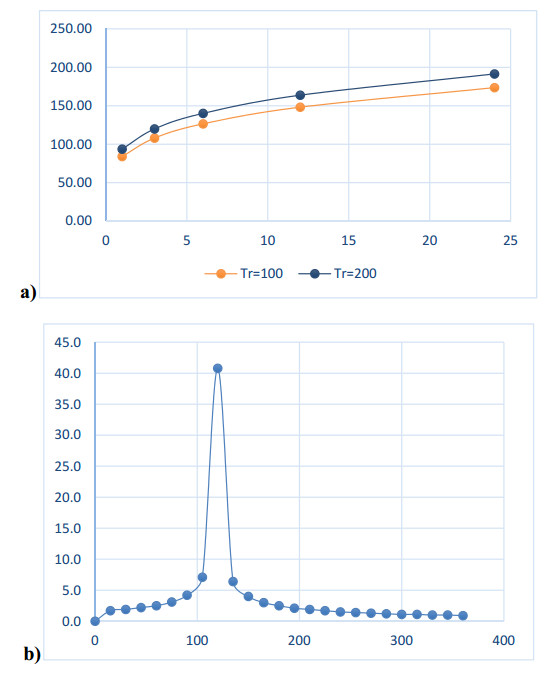
The present work, by applying the Gumbel distribution (Generalized Extreme Value Type-I distribution) on two rainfall series (1951–2018 and 1998–2018) coming from the same rain gauges and the "Chicago Method" for the calculation of the design storm, highlights how the choice of the series may influence the formation of flood events.
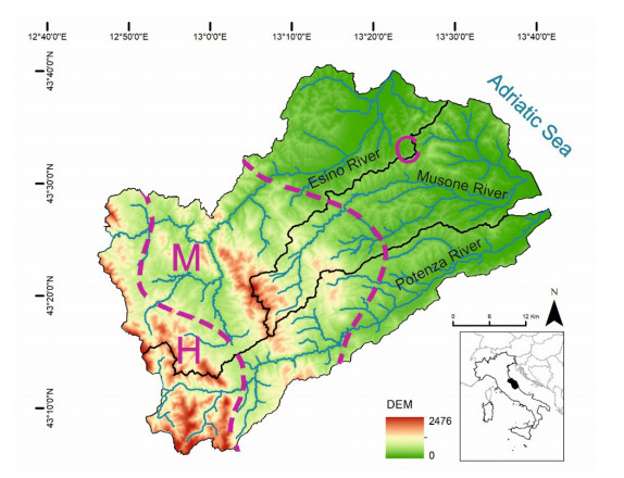
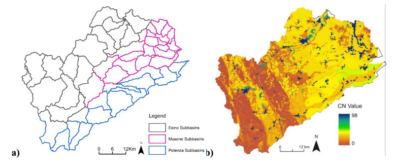
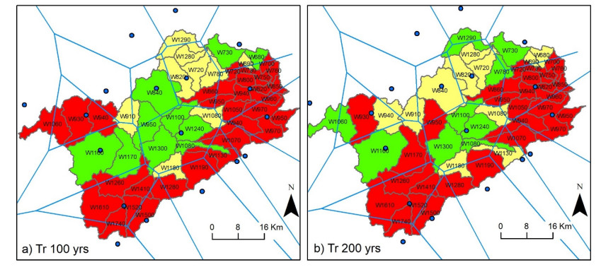
More in particular, the comparison of different hydrological models, generated using HEC-HMS software on three sample basins of the Adriatic side of central Italy, shows that the use of shorter and recent rainfall series results in a generally higher runoff, mostly in case of events with a return time equal or higher than 100 years.
Citation: Margherita Bufalini, Farabollini Piero, Fuffa Emy, Materazzi Marco, Pambianchi Gilberto, Tromboni Michele. The significance of recent and short pluviometric time series for the assessment of flood hazard in the context of climate change: examples from some sample basins of the Adriatic Central Italy[J]. AIMS Geosciences, 2019, 5(3): 568-590. doi: 10.3934/geosci.2019.3.568
Numerical hydrological models are increasingly a fundamental tool for the analysis of floods in a river basin. If used for predictive purposes, the choice of the "design storm" to be applied, once set other variables (as basin geometry, land use, etc.), becomes fundamental.
All the statistical methods currently adopted to calculate the design storm, suggest the use of long rainfall series (at least 40–50 years). On the other hand, the increasingly high frequency of intense events (rainfalls and floods) in the last twenty years, also as a result of the ongoing climate change, testify to the need for a critical analysis of the statistical significance of these methods.
The present work, by applying the Gumbel distribution (Generalized Extreme Value Type-I distribution) on two rainfall series (1951–2018 and 1998–2018) coming from the same rain gauges and the "Chicago Method" for the calculation of the design storm, highlights how the choice of the series may influence the formation of flood events.
More in particular, the comparison of different hydrological models, generated using HEC-HMS software on three sample basins of the Adriatic side of central Italy, shows that the use of shorter and recent rainfall series results in a generally higher runoff, mostly in case of events with a return time equal or higher than 100 years.

| [1] | Masson-Delmotte V, Zhai P, Pörtner H, et al. (2018) An IPCC Special Report on the impacts of global warming of 1.5 ℃ above pre-industrial levels and related global greenhouse gas emission pathways, in the context of strengthening the global response to the threat of climate change, sustainable development, 24. |
| [2] |
Huong HTL, Pathirana A (2013) Urbanization and climate change impacts on future urban flooding in Can Tho city, Vietnam. Hydrol Earth Syst Sci 17: 379–394. doi: 10.5194/hess-17-379-2013

|
| [3] |
Sperotto A, Torresan S, Gallina V, et al. (2016) A multi-disciplinary approach to evaluate pluvial floods risk under changing climate: The case study of the municipality of Venice (Italy). Sci Total Environ 562: 1031–1043. doi: 10.1016/j.scitotenv.2016.03.150
|
| [4] | Amici M, Spina R (2002) Campo medio della precipitazione annuale e stagionale sulle Marche per il periodo 1950–2000, 103. |
| [5] | Gentilucci M, Bisci C, Burt P, et al. (2018) Interpolation of Rainfall through Polynomial Regression in the Marche Region (Central Italy), Springer International Publishing. |
| [6] |
Pierantoni P, Deiana G, Galdenzi S (2013) Stratigraphic and structural features of the sibillini mountains(Umbria- Marche Apennines, Italy). Ital J Geosci 132: 497–520. doi: 10.3301/IJG.2013.08
|
| [7] |
Gumbel EJ (1941) Probability‐interpretation of the observed return‐periods of floods. Eos, Trans Am Geophys Union 22: 836–850. doi: 10.1029/TR022i003p00836
|
| [8] | Gumbel EJ (1954) Statistical theory of extreme values and some practical applications. Appl Math Ser 33: 341–342. |
| [9] |
Tabari H, Talaee PH (2011) Analysis of trends in temperature data in arid and semi-arid regions of Iran. Glob Planet Change 79: 1–10. doi: 10.1016/j.gloplacha.2011.07.008
|
| [10] |
Gocic M, Trajkovic S (2013) Analysis of changes in meteorological variables using Mann-Kendall and Sen's slope estimator statistical tests in Serbia. Glob Planet Change 100: 172–182. doi: 10.1016/j.gloplacha.2012.10.014
|
| [11] | Thiessen AH (1911) Precipitation for large areas. Mon Weather Rev 39: 1082–1084. |
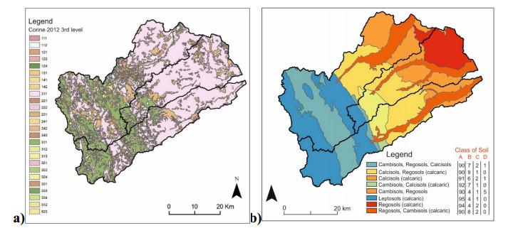
| [12] | NBGC (2006) Valter Sambucini, Ines Marinosci, CORINE LAND COVER 2006 (ISPRA). |
| [13] | Food and Agriculture Organization of the United Nations (2015) International soil classification system for naming soils and creating legends for soil maps. |
| [14] | USDA-NRCS (2009) National Engineering Handbook Chapter 7: Hydrologic Soil Groups. Part 630 Hydrol Natl Eng Handb, 5. |
| [15] | Fleming MJ, Doan JH (2013) HEC-GeoHMS geospatial hydrologic modeling extension. |
| [16] | Scharffenberg B, Bartles M, Brauer T, et al. (2018) Hydrologic Modeling System User's Manual. |
| [17] | USDA-NRCS (2009) Hydrology National Engineering Handbook Chapter 10 Estimation of Direct Runoff from Storm Rainfall. Part 630 Hydrol Natl Eng Handb. |
Figures(8) / Tables(13)

Margherita Bufalini, Farabollini Piero, Fuffa Emy, Materazzi Marco, Pambianchi Gilberto, Tromboni Michele. The significance of recent and short pluviometric time series for the assessment of flood hazard in the context of climate change: examples from some sample basins of the Adriatic Central Italy[J]. AIMS Geosciences, 2019, 5(3): 568-590. doi: 10.3934/geosci.2019.3.568


 DownLoad: