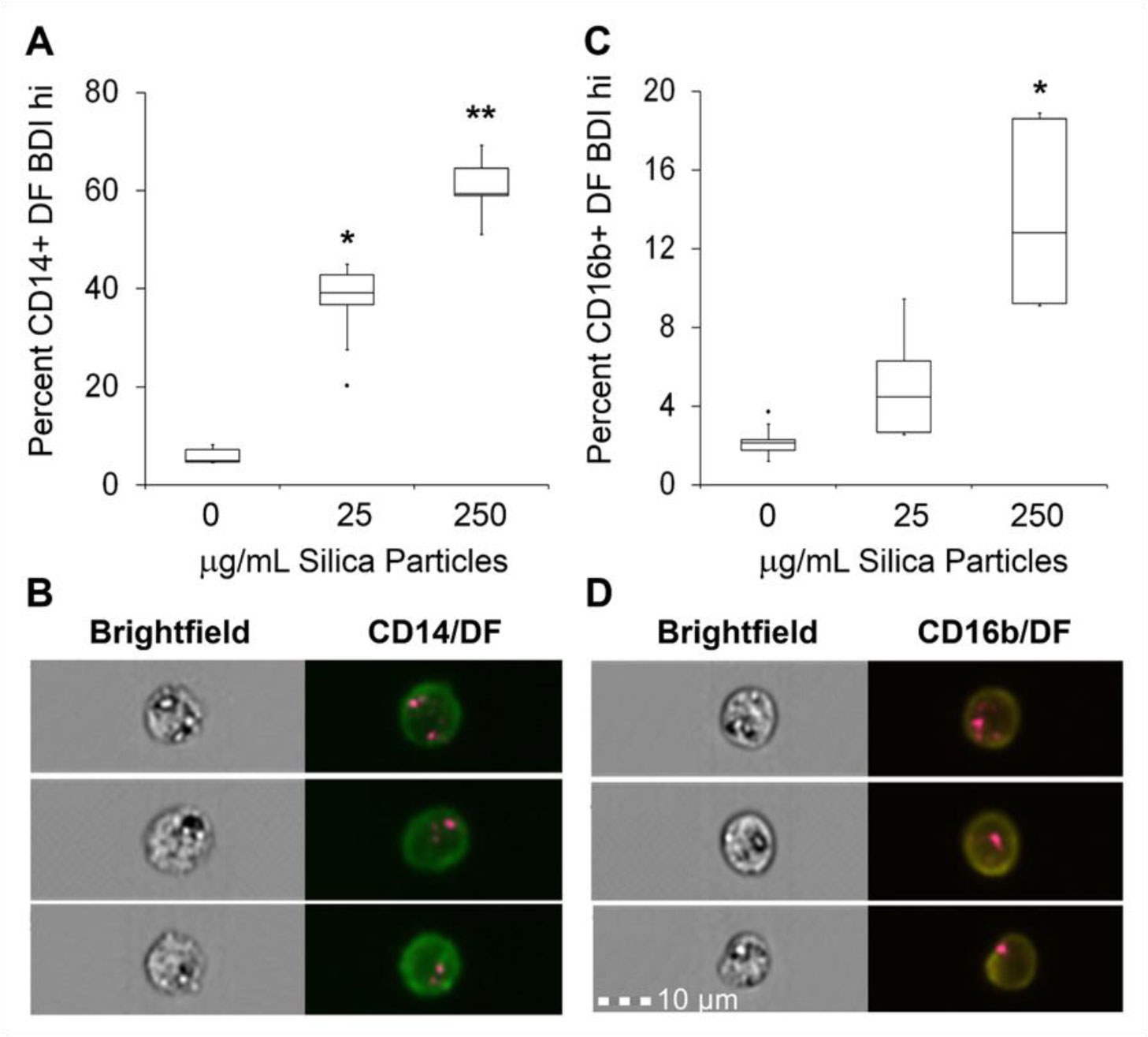
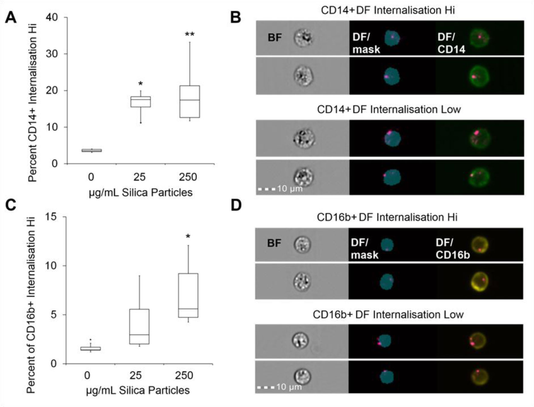
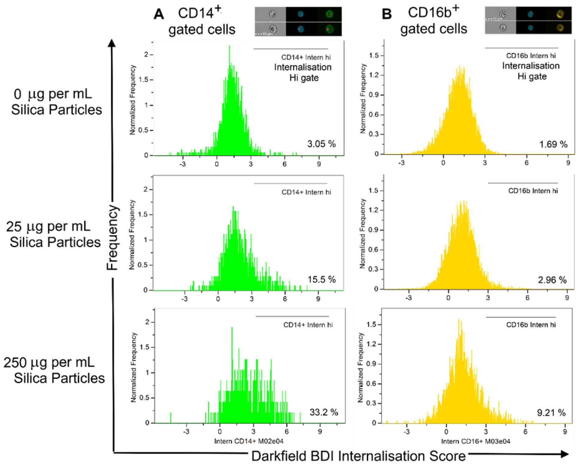
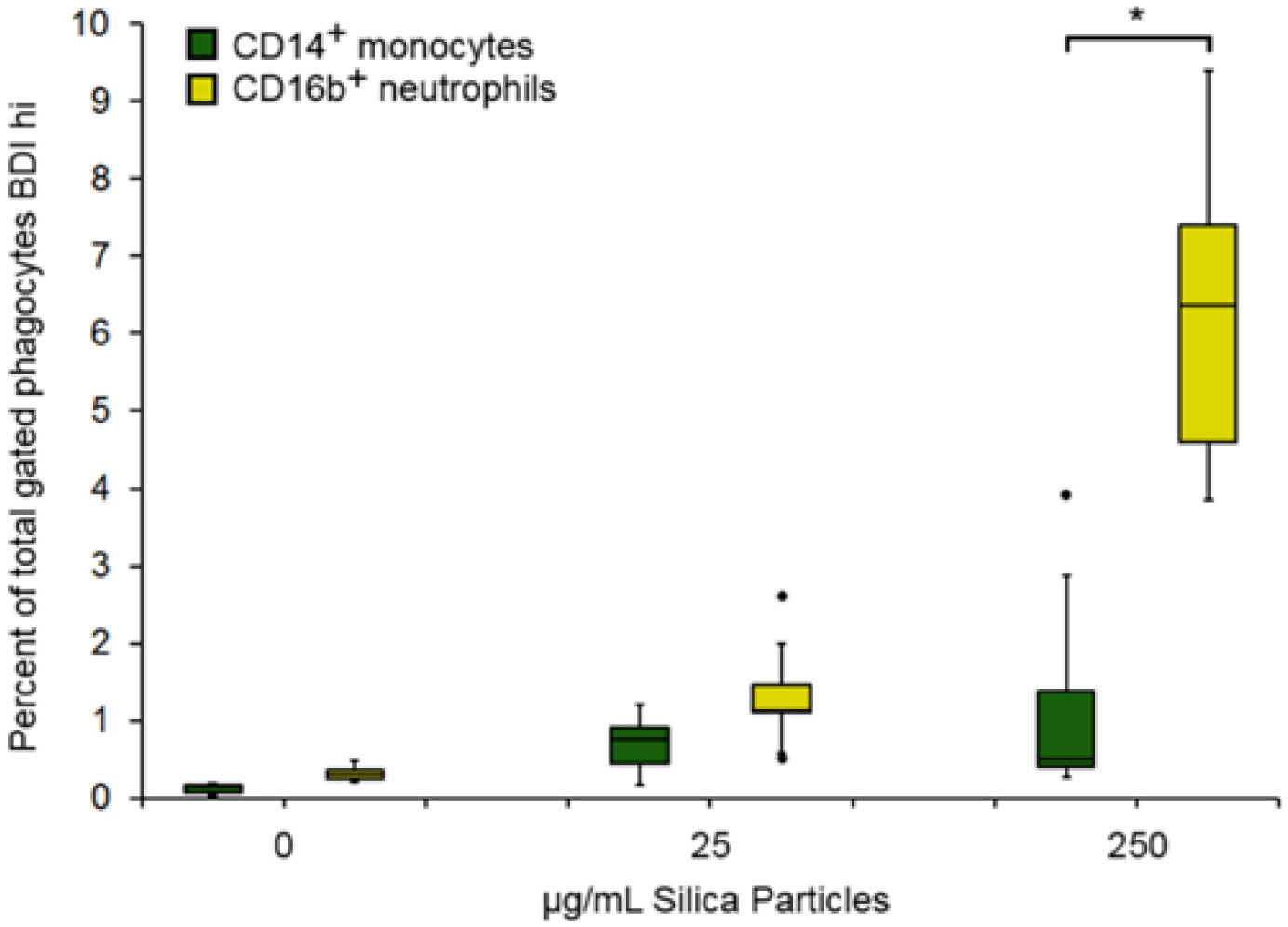
Exposure to respirable fractions of crystalline silica quartz dust particles is associated with silicosis, cancer and the development of autoimmune conditions. Early cellular interactions are not well understood, partly due to a lack of suitable technological methods. Improved techniques are needed to better quantify and study high-level respirable crystalline silica exposure in human populations. Techniques that can be applied to complex biological matrices are pivotal to understanding particle-cell interactions and the impact of particles within real, biologically complex environments. In this study, we investigated whether imaging flow cytometry could be used to assess the interactions between cells and crystalline silica when present within complex biological matrices. Using the respirable-size fine quartz crystalline silica dust Min-u-sil® 5, we first validated previous reports that, whilst associating with cells, crystalline silica particles can be detected solely through their differential light scattering profile using conventional flow cytometry. This same property reliably identified crystalline silica in association with primary monocytic cells in vitro using an imaging flow cytometry assay, where darkfield intensity measurements were able to detect crystalline silica concentrations as low as 2.5 µg/mL. Finally, we ultilised fresh whole blood as an exemplary complex biological matrix to test the technique. Even after the increased sample processing required to analyse cells within whole blood, imaging flow cytometry was capable of detecting and assessing silica-association to cells. As expected, in fresh whole blood exposed to crystalline silica, neutrophils and cells of the monocyte/macrophage lineage phagocytosed the particles. In addition to the use of this technique in in vitro exposure models, this method has the potential to be applied directly to ex vivo diagnostic studies and research models, where the identification of crystalline silica association with cells in complex biological matrices such as bronchial lavage fluids, alongside additional functional and phenotypic cellular readouts, is required.
Citation: Bradley Vis, Jonathan J. Powell, Rachel E. Hewitt. Imaging flow cytometry methods for quantitative analysis of label-free crystalline silica particle interactions with immune cells[J]. AIMS Biophysics, 2020, 7(3): 144-166. doi: 10.3934/biophy.2020012
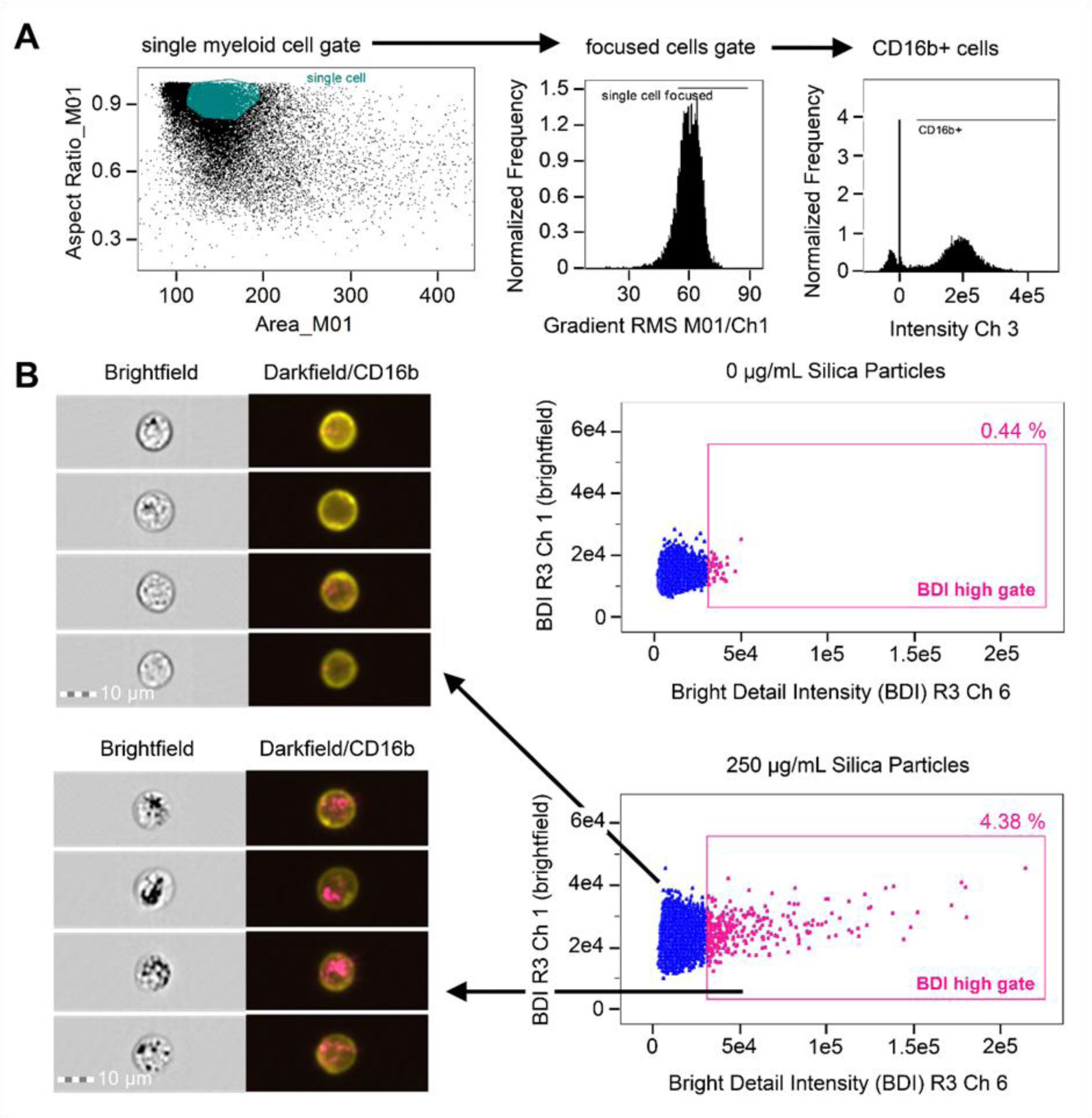
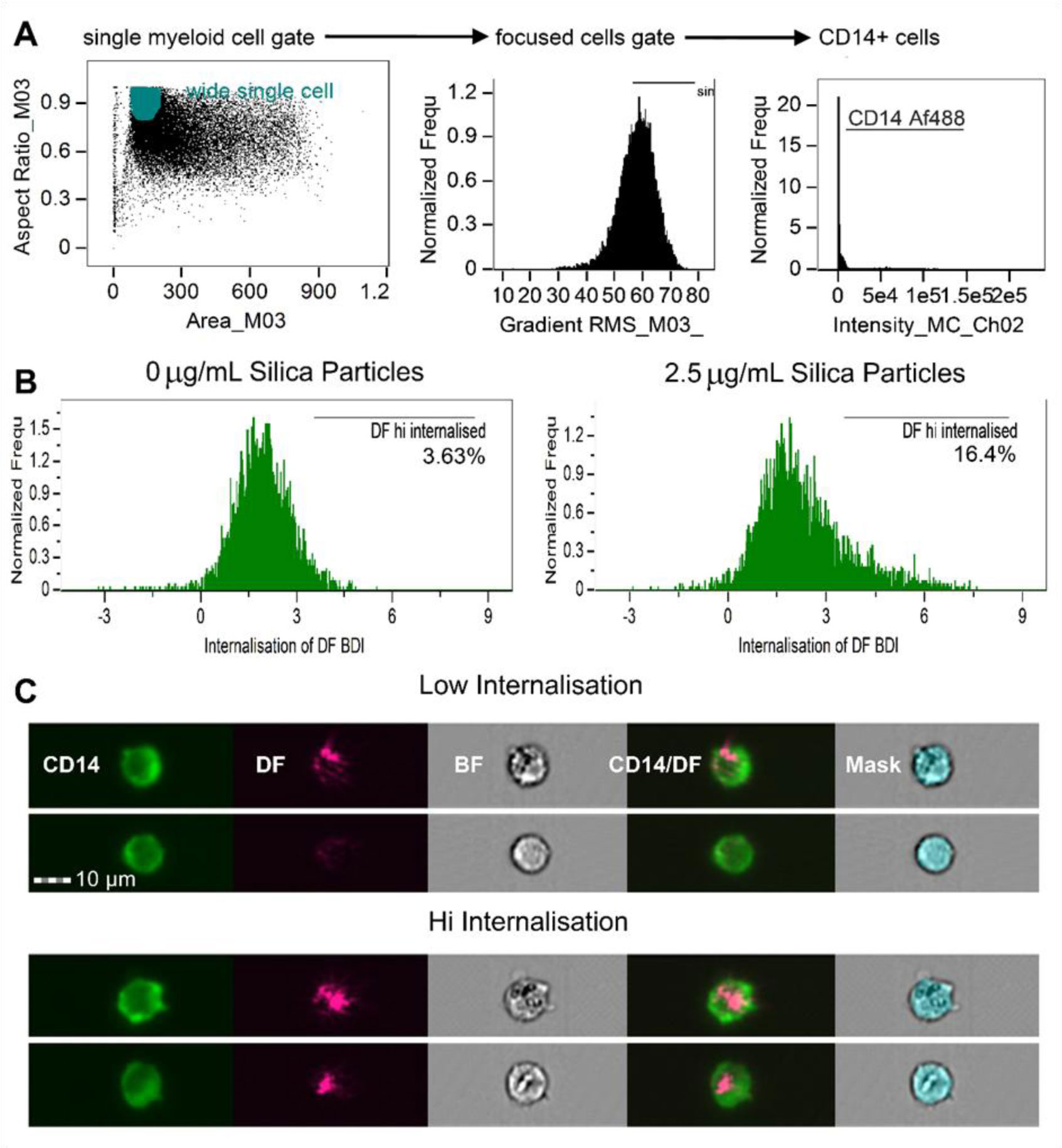
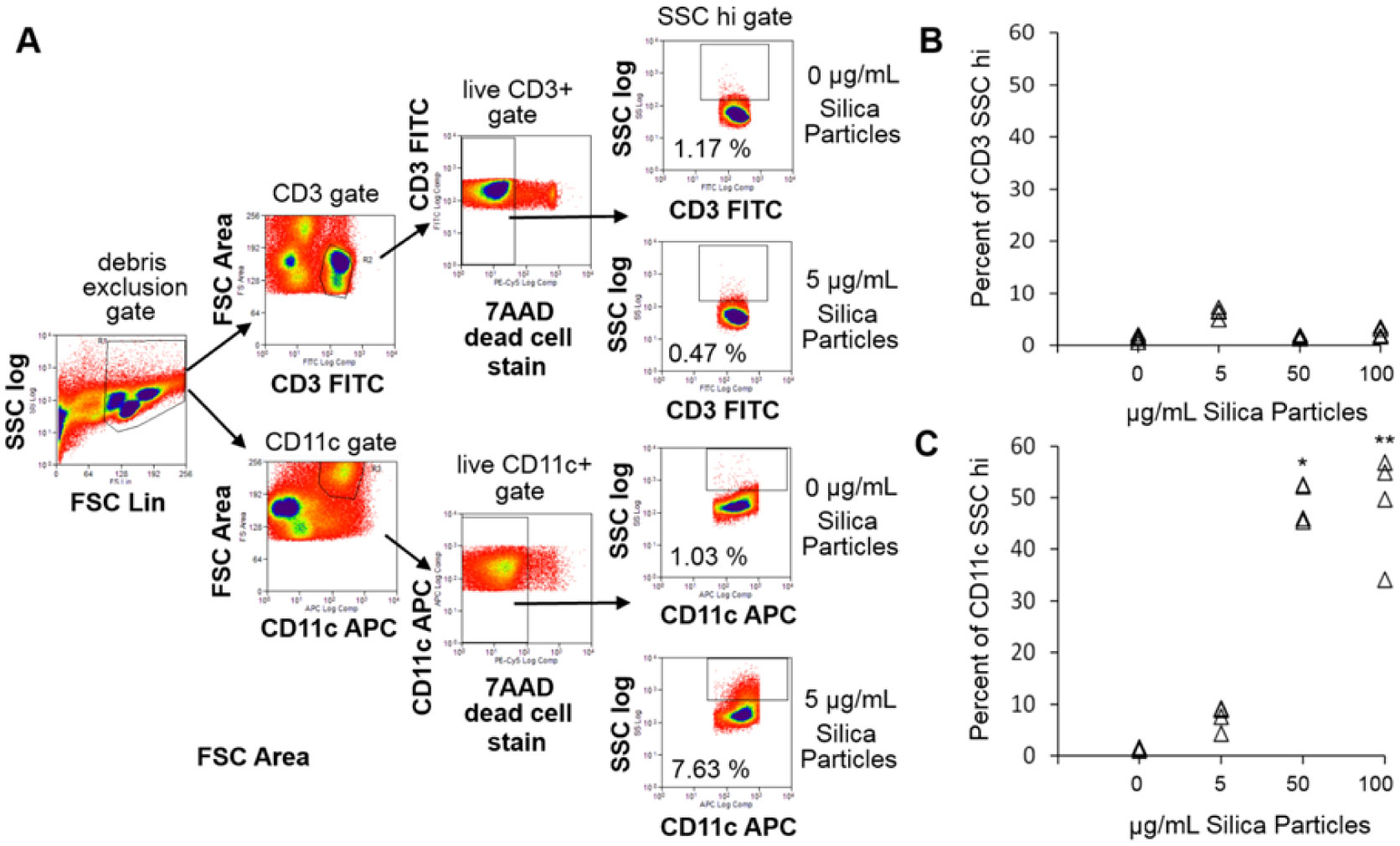
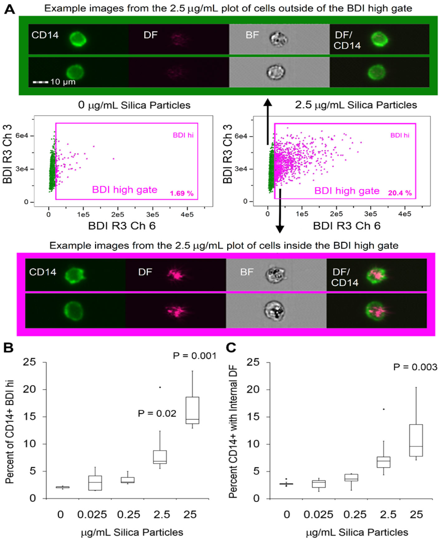
Exposure to respirable fractions of crystalline silica quartz dust particles is associated with silicosis, cancer and the development of autoimmune conditions. Early cellular interactions are not well understood, partly due to a lack of suitable technological methods. Improved techniques are needed to better quantify and study high-level respirable crystalline silica exposure in human populations. Techniques that can be applied to complex biological matrices are pivotal to understanding particle-cell interactions and the impact of particles within real, biologically complex environments. In this study, we investigated whether imaging flow cytometry could be used to assess the interactions between cells and crystalline silica when present within complex biological matrices. Using the respirable-size fine quartz crystalline silica dust Min-u-sil® 5, we first validated previous reports that, whilst associating with cells, crystalline silica particles can be detected solely through their differential light scattering profile using conventional flow cytometry. This same property reliably identified crystalline silica in association with primary monocytic cells in vitro using an imaging flow cytometry assay, where darkfield intensity measurements were able to detect crystalline silica concentrations as low as 2.5 µg/mL. Finally, we ultilised fresh whole blood as an exemplary complex biological matrix to test the technique. Even after the increased sample processing required to analyse cells within whole blood, imaging flow cytometry was capable of detecting and assessing silica-association to cells. As expected, in fresh whole blood exposed to crystalline silica, neutrophils and cells of the monocyte/macrophage lineage phagocytosed the particles. In addition to the use of this technique in in vitro exposure models, this method has the potential to be applied directly to ex vivo diagnostic studies and research models, where the identification of crystalline silica association with cells in complex biological matrices such as bronchial lavage fluids, alongside additional functional and phenotypic cellular readouts, is required.

| [1] | (1997) World Health OrganizationSilica, some silicates, coal dust and para-aramid fibrils. IARC Monographs on the Evaluation of Carcinogenic Risks to Humans . Lyon: IARC Press. |
| [2] | Health and Safety Executive Research Report RR878 - Levels of respirable dust and respirable crystalline silica at construction sites.Available from: https://www.hse.gov.uk/research/rrhtm/rr878.htm. |
| [3] | World Health Organization (2000) Crystalline Silica, Quartz (Concise International Chemical Assessment Document 24), ISBN-10: 9241530243.Available from: http://www.inchem.org/documents/cicads/cicads/cicad24.htm. |
| [4] |
Pollard KM (2016) Silica, Silicosis, and Autoimmunity. Front Immunol 7: 97. doi: 10.3389/fimmu.2016.00097

|
| [5] |
Miller FW, Alfredsson L, Costenbader KH, et al. (2012) Epidemiology of environmental exposures and human autoimmune diseases: findings from a National Institute of Environmental Health Sciences Expert Panel Workshop. J Autoimmun 39: 259-271. doi: 10.1016/j.jaut.2012.05.002
|
| [6] |
Bartůňková J, Pelclova D, Fenclová Z, et al. (2006) Exposure to silica and risk of ANCA-associated vasculitis. Am J Ind Med 49: 569-576. doi: 10.1002/ajim.20327
|
| [7] |
Pollard KM, Hultman P, Kono DH (2010) Toxicology of autoimmune diseases. Chem Res Toxicol 23: 455-466. doi: 10.1021/tx9003787
|
| [8] |
Lee S, Matsuzaki H, Kumagai-Takei N, et al. (2014) Silica exposure and altered regulation of autoimmunity. Environ Health Prev Med 19: 322-329. doi: 10.1007/s12199-014-0403-9
|
| [9] |
Van der Woude FJ, Lobatto S, Permin H, et al. (1985) Autoantibodies against neutrophils and monocytes. Tool for diagnosis and marker of disease activity in Wegener's granulomatosis. Lancet 325: 425-429. doi: 10.1016/S0140-6736(85)91147-X
|
| [10] |
Germolec D, Kono DH, Pfau JC, et al. (2012) Animal models used to examine the role of the environment in the development of autoimmune disease: findings from an NIEHS Expert Panel Workshop. J Autoimmun 39: 285-293. doi: 10.1016/j.jaut.2012.05.020
|
| [11] |
Riediker M, Zink D, Kreyling W, et al. (2019) Particle toxicology and health-where are we? Part Fibre Toxicol 16: 19. doi: 10.1186/s12989-019-0302-8
|
| [12] |
Murphy CJ, Vartanian AM, Geiger FM, et al. (2015) Biological responses to engineered nanomaterials: Needs for the next decade. ACS Central Sci 1: 117-123. doi: 10.1021/acscentsci.5b00182
|
| [13] |
Fröhlich E (2015) Value of phagocyte function screening for immunotoxicity of nanoparticles in vivo. Int J Nanomed 10: 3761-3778. doi: 10.2147/IJN.S83068
|
| [14] |
Jochums A, Friehs E, Sambale F, et al. (2017) Revelation of Different Nanoparticle-Uptake Behavior in Two Standard Cell Lines NIH/3T3 and A549 by Flow Cytometry and Time-Lapse Imaging. Toxics 5: 15. doi: 10.3390/toxics5030015
|
| [15] |
Parks CG, Miller FW, Pollard KM, et al. (2014) Expert panel workshop consensus statement on the role of the environment in the development of autoimmune disease. Int J Mol Sci 15: 14269-14297. doi: 10.3390/ijms150814269
|
| [16] |
Baumann D, Hofmann D, Nullmeier S, et al. (2013) Complex encounters: nanoparticles in whole blood and their uptake into different types of white blood cells. Nanomedicine 8: 699-713. doi: 10.2217/nnm.12.111
|
| [17] |
Vranic S, Boggetto N, Contremoulins V, et al. (2013) Deciphering the mechanisms of cellular uptake of engineered nanoparticles by accurate evaluation of internalization using imaging flow cytometry. Part Fibre Toxicol 10: 2. doi: 10.1186/1743-8977-10-2
|
| [18] | Phanse Y, Ramer-Tait AE, Friend SL, et al. (2012) Analyzing cellular internalization of nanoparticles and bacteria by multi-spectral imaging flow cytometry. J Vis Exp 64: e3884. |
| [19] |
Rieger AM, Hall BE, Barreda DR (2010) Macrophage activation differentially modulates particle binding, phagocytosis and downstream antimicrobial mechanisms. Dev Comp Immunol 34: 1144-1159. doi: 10.1016/j.dci.2010.06.006
|
| [20] | Marangon I, Boggetto N, Ménard-Moyon C, et al. (2013) Localization and relative quantification of carbon nanotubes in cells with multispectral imaging flow cytometry. J Vis Exp 82: e50566. |
| [21] |
Smirnov A, Solga MD, Lannigan J, et al. (2015) An improved method for differentiating cell-bound from internalized particles by imaging flow cytometry. J Immunol Methods 423: 60-69. doi: 10.1016/j.jim.2015.04.028
|
| [22] |
Tian L, Dai S, Wang J, et al. (2008) Nanoquartz in Late Permian C1 coal and the high incidence of female lung cancer in the Pearl River Origin area: a retrospective cohort study. BMC Public Health 8: 398. doi: 10.1186/1471-2458-8-398
|
| [23] |
Hornung V, Bauernfeind F, Halle A, et al. (2008) Silica crystals and aluminum salts activate the NALP3 inflammasome through phagosomal destabilization. Nat Immunol 9: 847-856. doi: 10.1038/ni.1631
|
| [24] |
Beamer CA, Holian A (2005) Scavenger receptor class A type I/II (CD204) null mice fail to develop fibrosis following silica exposure. Am J Physiol Lung Cell Mol Physiol 289: L186-L195. doi: 10.1152/ajplung.00474.2004
|
| [25] |
Beamer GL, Seaver BP, Jessop F, et al. (2016) Acute exposure to crystalline silica reduces macrophage activation in response to bacterial lipoproteins. Front Immunol 7: 49. doi: 10.3389/fimmu.2016.00049
|
| [26] | Schorn C, Janko C, Latzko M, et al. (2012) Monosodium urate crystals induce extracellular DNA traps in neutrophils, eosinophils, and basophils but not in mononuclear cells. Front Immunol 3: 277. |
| [27] |
Satpathy SR, Jala VR, Bodduluri SR, et al. (2015) Crystalline silica-induced leukotriene B4-dependent inflammation promotes lung tumour growth. Nat Commun 6: 7064. doi: 10.1038/ncomms8064
|
| [28] |
Chubb LG, Cauda EG (2017) Characterizing particle size distributions of crystalline silica in gold mine dust. Aerosol Air Qual Res 17: 24-33. doi: 10.4209/aaqr.2016.05.0179
|
| [29] |
Dominical V, Samsel L, McCoy JP (2017) Masks in imaging flow cytometry. Methods 112: 9-17. doi: 10.1016/j.ymeth.2016.07.013
|
| [30] |
Boyette LB, Macedo C, Hadi K, et al. (2017) Phenotype, function, and differentiation potential of human monocyte subsets. PLoS One 12: e0176460. doi: 10.1371/journal.pone.0176460
|
| [31] |
Rosales C (2018) Neutrophil: A cell with many roles in inflammation or several cell types? Front Physiol 9: 113. doi: 10.3389/fphys.2018.00113
|
| [32] |
Hewitt RE, Vis B, Pele LC, et al. (2017) Imaging flow cytometry assays for quantifying pigment grade titanium dioxide particle internalization and interactions with immune cells in whole blood. Cytom Part A 91: 1009-1020. doi: 10.1002/cyto.a.23245
|
| [33] |
Sellamuthu R, Umbright C, Roberts JR, et al. (2011) Blood gene expression profiling detects silica exposure and toxicity. Toxicol Sci 122: 253-264. doi: 10.1093/toxsci/kfr125
|
| [34] |
Ishihara Y, Yasuhara T, Ishiyama S, et al. (2001) The role of leukocytes during acute phase inflammation in crystalline silica-induced lung injury. Exp Lung Res 27: 589-603. doi: 10.1080/019021401753181845
|
| [35] |
Baldwin PEJ, Yates T, Beattie H, et al. (2019) Exposure to Respirable Crystalline Silica in the GB Brick Manufacturing and Stone Working Industries. Ann Work Expos Health 63: 184-196. doi: 10.1093/annweh/wxy103
|
| [36] | Künzli N, Perez L, Rapp R (2010) Air quality and health. Lausanne: European Respiratory Society. World Health Organ 89. |
| [37] |
Schmid O, Cassee FR (2017) On the pivotal role of dose for particle toxicology and risk assessment: exposure is a poor surrogate for delivered dose. Part Fibre Toxicol 14: 52. doi: 10.1186/s12989-017-0233-1
|
| [38] |
Fröhlich E, Mercuri A, Wu S, et al. (2016) Measurements of deposition, lung surface area and lung fluid for simulation of inhaled compounds. Front Pharmacol 7: 181. doi: 10.3389/fphar.2016.00181
|
| [39] |
Friedetzky A, Garn H, Kirchner A, et al. (1998) Histopathological changes in enlarged thoracic lymph nodes during the development of silicosis in rats. Immunobiology 199: 119-132. doi: 10.1016/S0171-2985(98)80068-5
|
| [40] |
Xu M, Qing M, Peng D (2014) Silicon dioxide particles deposited in vessels and cartilage of the femoral head. Yonsei Med J 55: 1447-1449. doi: 10.3349/ymj.2014.55.5.1447
|
| [41] |
Slavin RE, Swedo JL, Brandes D, et al. (1985) Extrapulmonary silicosis: a clinical, morphologic, and ultrastructural study. Hum Pathol 16: 393-412. doi: 10.1016/S0046-8177(85)80233-1
|
| [42] |
Chu Z, Huang Y, Li L, et al. (2012) Physiological pathway of human cell damage induced by genotoxic crystalline silica nanoparticles. Biomaterials 33: 7540-7546. doi: 10.1016/j.biomaterials.2012.06.073
|
| [43] | Ueki A, Yamaguchi M, Ueki H, et al. (1994) Polyclonal human T-cell activation by silicate in vitro. Immunology 82: 332. |
| [44] |
Wu P, Hyodoh F, Hatayama T, et al. (2005) Induction of CD69 antigen expression in peripheral blood mononuclear cells on exposure to silica, but not by asbestos/chrysotile-A. Immunol Lett 98: 145-152. doi: 10.1016/j.imlet.2004.11.005
|
| [45] |
Braakhuis HM, Park MVDZ, Gosens I, et al. (2014) Physicochemical characteristics of nanomaterials that affect pulmonary inflammation. Part Fibre Toxicol 11: 18. doi: 10.1186/1743-8977-11-18
|
| [46] |
Vis B, Hewitt RE, Faria N, et al. (2018) Non-functionalized ultrasmall silica nanoparticles directly and size-selectively activate T cells. ACS Nano 12: 10843-10854. doi: 10.1021/acsnano.8b03363
|
| [47] |
Vis B, Hewitt RE, Monie TP, et al. (2020) Ultrasmall silica nanoparticles directly ligate the T cell receptor complex. P Natl Acad Sci 117: 285-291. doi: 10.1073/pnas.1911360117
|
| [48] |
Eleftheriadis T, Pissas G, Zarogiannis S, et al. (2019) Crystalline silica activates the T-cell and the B-cell antigen receptor complexes and induces T-cell and B-cell proliferation. Autoimmunity 52: 136-143. doi: 10.1080/08916934.2019.1614171
|
| [49] |
Hewitt RE, Chappell HF, Powell JJ (2020) Small and dangerous? Potential toxicity mechanisms of common exposure particles and nanoparticles. Curr Opin Toxicol 19: 93-98. doi: 10.1016/j.cotox.2020.01.006
|
| [50] |
Gilberti RM, Joshi GN, Knecht DA (2008) The phagocytosis of crystalline silica particles by macrophages. Am J Resp Cell Mol Biol 39: 619-627. doi: 10.1165/rcmb.2008-0046OC
|
| [51] |
Pacheco P, White D, Sulchek T (2013) Effects of microparticle size and Fc density on macrophage phagocytosis. PLoS One 8: e60989. doi: 10.1371/journal.pone.0060989
|
| [52] | Dale DC, Boxer L, Liles WC (2008) The phagocytes: neutrophils and monocytes. Blood, J Am Soc Hematol 112: 935-945. |
| [53] |
Brinkmann V, Zychlinsky A (2012) Neutrophil extracellular traps: is immunity the second function of chromatin? J Cell Biol 198: 773-783. doi: 10.1083/jcb.201203170
|
| [54] |
Desai J, Foresto-Neto O, Honarpisheh M, et al. (2017) Particles of different sizes and shapes induce neutrophil necroptosis followed by the release of neutrophil extracellular trap-like chromatin. Sci Rep 7: 15003. doi: 10.1038/s41598-017-15106-0
|
 biophy-07-03-012-s001.pdf biophy-07-03-012-s001.pdf |
 |
Figures(9)

Bradley Vis, Jonathan J. Powell, Rachel E. Hewitt. Imaging flow cytometry methods for quantitative analysis of label-free crystalline silica particle interactions with immune cells[J]. AIMS Biophysics, 2020, 7(3): 144-166. doi: 10.3934/biophy.2020012


 DownLoad: